Five time sequence prediction of deep learning model comparison summary: from simulation statistics models to pre -training unsupervised models (attached code)

Source: Deephub IMBA

This article is about 6700 words, it is recommended to read for 12 minutes

This article discusses five deep learning architectures that specialize in time sequence prediction.

Time sequence prediction has undergone tremendous changes in the past two years. Especially after the emergence of Kaiming's MAE, the model of the time sequence can also be used in unsupervised pre -training in a method similar to MAE.

Makridakis M-Competitions series (known as M4 and M5, respectively) in 2018 and 2020 (M6 was also held this year). For those who do not understand, the M series can be considered a summary of the existing state of the time sequence ecosystem, providing experience and objective evidence for the current predicted theory and practice.

The results of M4 in 2018 show that the pure "ML" method is largely better than traditional statistical methods, which was unexpected at the time. In the M5 [1] two years later, the most high score is only the "ML" method. And all the top 50 are basically ML (mostly tree models). This game saw the first appearance of LightGBM (for time sequence prediction) and Amazon's Deepar [2] and N-Beats [3]. The N-Beats model was released in 2020, and the winner of the M4 competition was 3 %!

The recent Ventilator Pressure Prediction competition shows the importance of using deep learning methods to cope with real -time time sequence challenges. The purpose of the competition is to predict the sequence of the stress of mechanical lungs. Each training instance is its own time sequence, so the task is a problem of multiple time sequences. The winning team submits a multi -layered depth architecture, including LSTM networks and Transformer blocks.

In the past few years, many famous architectures have been released, such as MQRNN and DSSM. All these models use deep learning to contribute many new things to the field of time series prediction. In addition to winning the Kaggle competition, we have also brought us more progress, such as::

Multi -functional: The ability to use the model for different tasks.

Mlop: The ability to use models in production.

Explanation and explanation: The black box model is not so popular.

This article discusses 5 deep learning architectures that specialize in time sequence prediction. The thesis is:

N-Beats (Elementai)

Deepar (amazon)

SpaceTimeFormer [4]

Temporal Fusion Transformer or TFT (Google) [5]

TSFormer (MAE in the Time Series) [7]

N-eeats

This model directly comes from Elementai (unfortunate) short -lived Elementai, which was founded by Yoshua Bengio. The top architecture and its main components are shown in Figure 1:

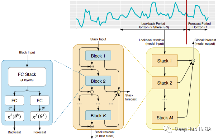
N-Beats is a pure deep learning architecture. It is based on the deep stack of the integrated feeding network. These networks also stack through positive and reverse interconnection.

Each block only models the residue generated by the previous backcast, and then predicts based on the error update. This process simulates the Box-Jenkins method when fitting ARIMA models.

The following is the main advantage of this model:

Expressive and easy to use: This model is easy to understand, with a modular structure. It is designed as the minimum time sequence feature engineering and does not need to be scaled to input.

This model has the ability to summarize multiple time sequences. In other words, the distribution has a slightly different time sequence that can be used as input. In N-Beats, it is achieved through meta-learning. The Yuan learning process includes two processes: internal learning and external learning processes. The internal learning process occurs in the block and helps the model capture local time characteristics. The external learning process occurs at the stack layer to help the global characteristics of all time sequences in the model learning.

Double residual superposition: The idea of ​​residual connection and superposition is very clever, and it is almost used for the deep neural network of each type. The same principle is applied in the implementation of N-Beats, but there are some additional modifications: each block has two residual branches, one runs in the backing window (called backcast), and the other runs in the forecast window (called For Forecast).

Each continuous block only models the residues generated by the previous block rebuilding, and then updates prediction based on the error. This helps the model to better approach the useful post -push signal. At the same time, the final stack prediction prediction is being modeling as a layered hierarchy of all parts of the prediction. This is the BOX-JENKINS method of the Arima model.

Explaining: There are two variants in the model, general and explanatory. In general variants, the final right value of the full connection layer of each block is learned at the general variant. In explained variants, the last layer of each block is deleted. Then push the backbackcast and predict the ForeCast branch multiplied to simulate the specific matrix of the analog trend (monotonous function) and seasonal (cyclical cycle function). Note: The original N-Beats implementation is only suitable for single-variable time sequence.

Deepar

Based on a novel time sequence model with deep learning and self -regression characteristics. Figure 2 shows the top architecture of Deepar:

The following is the main advantage of this model:

Deepar works very well on multiple time sequences: to build a global model by using multiple distributions with different time sequences. It is also suitable for many realistic scenarios. For example, power companies may want to launch electric prediction services for each customer, and each customer has different consumption models (which means different distributions).

In addition to historical data, Deepar also allows the use of known future time sequences (a feature of a self -regression model) and additional static attributes. In the previously mentioned electric demand prediction scenario, an additional time variable can be a month (as an integer, between 1-12). Assuming that each customer is associated with a sensor that measures power consumption, then the additional static variables will be things like Sensor_id or Customer_id.

If you do n’t know the use of neural network architecture such as MLPS and RNN for time sequence prediction, then a key pre -processing step is to use standardized or standardized technologies to zoom in time sequence. This does not need to be manually operated in Deepar, because the underlying model of each time sequence I is zoomed in the self -regression input Z of each time sequence i. The zoom factor is V_i, that is, the average value of the time sequence. Specifically, the proportional factor equation used in the thesis benchmark is as follows:

However, in practice, if the size of the target time sequence is very different, it is necessary to apply its own zoom in the pre -processing process. For example, in the energy demand forecast scenario, the data set can include medium -voltage power customers (such as small factories, consumption of electricity according to the MW unit) and low -voltage customers (such as family, consumption of electricity according to the kilowatt unit).

Deepar perform probability prediction, not directly output the future value. This is completed in the form of Monte Carlo sample.

These predictions are used to calculate the segmentation prediction and use the segmentation loss function. For those who are unfamiliar with this type of loss, the loss of the division is not only used to calculate an estimate, but also to calculate the forecast interval around this value.

SpaceTimeFormer

Time dependencies in single variable time series are the most important. But in multiple time series scenarios, things are not so simple. For example, suppose we have a weather forecast task to predict the temperature of five cities. Let us assume that these cities belong to a country. In view of what we are currently seeing, we can use Deepar and model each city as an external static cooperative variable.

In other words, the model will consider time and space at the same time. This is the core concept of SpaceTimeFormer:

Use a model to use the spatial relationship between these cities/locations, so as to learn extra useful dependencies, because the model will consider time and spatial relationship at the same time.

In -depth study of time and space sequence

As the name suggests, this model uses a structure based on Transformers. When using a TranSFormers model for time sequence prediction, a popular time perception of time perception is to transmit input through Time2vec [6] embedded layer (for NLP tasks to use position encoding vectors to replace Time2vec). Although this technology is very effective for single -variable time sequences, it does not make any sense to the input of multiple variables. It may be in the language modeling. Each word in the sentence is embedded in embedded. The word is essentially a part of the vocabulary, and the time sequence is not so simple.

In the multi -time sequence, at the given time step -long T, the input form is x_1, t, x2, t, x_m, T, where x_i, t is the value of feature I, M is the total number of features/sequences. If we will enter a Time2VEC layer, it will generate a time to embed the vector. What does this embedded? The answer is that it will represent the entire input set as a single entity (token). Therefore, the model will only be dynamically dynamic between time steps, but the spatial relationship between features/variables will be missed.

SpaceTimeFormer solves this problem, which turns the input to a large vector and is called a space -time sequence. If the input contains n variables and is organized into a T -time step, the generated space -time sequence will be marked with (NXT). The following figure 3 shows this better:

The paper points out: "(1) contains a diverse input format of time information. The decoder input lacks ("? ") Value, and is set to zero when predicting. The frequency of the pattern is embedded. (3) binary embedding indicates whether the value is given as context or predictive. (4) reflect the integer index of each time sequence to a "space" with a search table embedded. ) Use the time2vec embedded and variable values ​​of each time sequence of the feeder layer. (6) the value and time, the variable and the given embedded sequential As an input. In other words, the final sequence encodes a uniform embedding that contains time, space, and context information. But a disadvantage of this method is that the sequence may become a long way to lead to the secondary growth of resources. Because according to the attention mechanism, each token must be checked for another. The author uses a more effective architecture, called Performer's attention mechanism, which is suitable for larger sequences.

Temporal Fusion Transformer

Temporal Fusion Transformer (TFT) is a TRANSFORMER -based time sequence prediction model released by Google. TFT is more common than previous models.

The top -level architecture of TFT is shown in Figure 4. The following is the main advantage of this model:

Like the model mentioned earlier, TFT supports build a model on multiple heterogeneous time sequences.

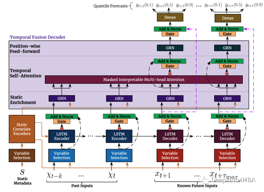
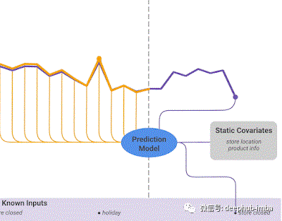
TFT supports three types of characteristics: i) The time -changing data II in the future input with known future input is only known to the time of time. Therefore, TFT is more common than the previous model. In the prediction scene mentioned earlier, we hope to use humidity levels as a time -changing feature, which is only known so far. This is feasible in TFT, but it can't work in Deepar.

Figure 5 shows how to use all these features::

TFT emphasizes interpretability. Specifically, by using the Variable Selection component (as shown in Figure 4 above), the model can successfully measure the impact of each characteristic. Therefore, it can be said that the model learns the importance of characteristics.

On the other hand, TFT proposes a new explanatory multi -attention mechanism: the weight of the attention of this layer can reveal which time is the most important time. The visualization of these weights can reveal the most significant season mode of the entire data concentration.

Forecasting interval: similar to Deepar, TFT returns the output prediction range and predictive values ​​by using the division number.

In summary, deep learning has undoubtedly changed the pattern of time series prediction. In addition to the unparalleled performance of the above models, there is also a common point: they make full use of multiple and diverse time data. At the same time, they use exogenous information to improve the predictive performance to unprecedented levels. However, most of the pre -training models are used in the Natural Language Treatment (NLP) task. FEEDs of NLP tasks are mostly data created by humans. They are full of rich and excellent information, which can almost be regarded as a data unit. In time sequence prediction, we can feel the lack of such pre -training models. Why can't we use this advantage in time sequences as in NLP?

This leads to the last model TSFormer we want to introduce. This model considers two perspectives. We say that from input to output to four parts, and provides Python implementation code (officially provided). This model is. Soon after it was released, we focused on it here.

TSFormer

It is an unsupervised time sequence pre -training model based on Transformer (TSFormer). It uses training strategies in MAE and can capture very long dependencies in data.

NLP and time series:

To some extent, NLP information is the same as Time Series data. They are all sequential data and local sensitivity, which means that it is related to its next/previous data point. But there are still some differences. When proposing our pre -training model, we should consider two differences, as we do in the NLP task:

The density of time sequence data is much lower than natural language data

We need longer time sequence data than NLP data

Introduction to TSFormer

The main architecture of TSFormer and MAE is basically similar. The data passes through a encoder and then passing through a decoder. The final goal is to rebuild data from missing (manual masking).

We summarize him as the following 4 points

1. cover

As a step into the encoder as a data. The input sequence (s 分) has been distributed in the P film, and its length is L. Therefore, Langth, a sliding window used for the next time, is P XL.

The shielding ratio is 75 % (it looks high, it is estimated that the parameters of the MAE are used); what we want to complete is a self -supervision task, so the less the data calculates the calculation speed, the faster.

The main reason for doing so (cover input sequence sequence) is:

Patch is better than individually.

It makes the use of downstream models simple (STGNN uses the unit segment as input)

You can decompose the input size of the encoder.

Class Patch (nn.module): Def __init __ (Self, Patch_size, input_Channel, Output_Channel, SPECTRAL = TRUE): <)/). code> self.output_channel = output_channel self.P = patch_size self.input_channel = input_channel self.output_channel = output_channel Self.spectral = SPECTRAL if spectral: Self.emb_layer = nn.linear (patch_size/2+1)*2, output_channel) Else: Self.input_embedding = nn.conv2d (input_Channel, Output_Channel, kernel_size = (Self.p, 1), Stride = (Self.p, 1)) > DEF FORWARD (SELF, Input): B, N, C, L = Input.shape if self.Spectral: SPEC_FEAT_ = TORCH.FFT.RFFT (input.unfold (-1, Self.p, Self.p), DIM = -1) Real = SPEC_FEAT_REAL Imag = SPEC_FEAT_.IMAG SPEC_FEAT = TORCH.CAT ([Real, Imag], DIM = -1) .squeeze (2) Output = Self.emb_layer (SPEC_FEAT) .transpose (-1, -2) Else: input = input.unsqueeze (-1) # b, n, c, l, 1 input = input.Reshape (b*n, C, L, 1) # B*N, C, L, 1 Output = Self.input_embedding (input) # b*n, d, l/p, 1 output = output.squeeze (-1) .View (B, N, Self.output_Channel, -1) assert output.shape [-1] == L/Self.p Code> Return Output

The following is a function that generates cover

Class Maskgenrator (nn.module): def __init __ (Self, Mask_size, Mask_ratio, Distribution = 'Uniform', LM = -1): super (super (super (super (super (super (super (super (super (super (supervisp>. __init __ () Self. Mask_size = Mask_size Self. Mask_ratio = Mask_ratio Self.sort = True Self.aVerage_PatChe_PatChe_PatChe_PatChe_Patche_PatChe_PatChe_Patche lm Self.distribution = Distribution If Self.distribution == "Geom": Assert LM! = -1 Assert distribution in ['geom', 'uniform'] defore uniform_rand (seld): Mask = list (range (seld.Mask_size ))) Random.shuffle (Mask) mask_len = int (seld.mask_size * self.mask_ratio) Self. Maskns = Mask_Len ] Self.unmasked_tokens = Mask [mask_len:] if self.sort: Self. Masked_tokens = sorted (seld.masoked_tokens) Self.unmasked_tok ENS = Sorted (Self.UnMasked_tokens) Return Self.unmasked_tokens, Self.Masked_tokens mask = geom_noise_mask_single(self.mask_size, lm=self.average_patch, masking_ratio=self.mask_ratio) # 1: masked, 0:unmasked self.masked_tokens = np.where(mask)[0].tolist () Self.unmasked_tokens = np.where (~ mask) [0] .tolist () # assert len ​​(self.masked_tokens) &

Len (Self.Unmasked_tokens) Return Self.unmasked_tokens, Self.MASKED_TOKENS deffard (seld): if Self .dribution == 'Geom': Self.unmasked_tokens, Self. Masked_tokens = Self.Geometric_rand () Self.Unmasked_tokens, Self. Masked_tokens = Self.uniform_RAND () Else: Raise Exception ("Error") Return Self. Masked_tokens 2. Code

Including input embedded, position coding and transformer block. The encoder can only be executed on the unobstructed patchs (this is also the method of the MAE).

Input embedded

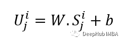
Use linear projection to obtain the input embedded, which can convert the unobstructed space into potential space. Its formula can be seen below:

W and B are learning parameters, U is the model input vector in the dimension.

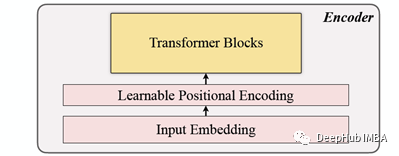
Position encoding

The simple position encoding layer is used to add new sequential information. Added the word "learning", which helps show better performance than sine. Therefore, the learning position embeds the good results of the time sequence.

Class LearnableTempoSitionalenCoding (nn.module): def __init __ (seld, d_model, dropout = 0.1, max_len: int (code> <). Self.dropout = nn.dropout (p = Dropout) Self.pe = nn.parameter (torch.empty (max_len, d_model) nn.init.uniform_ (Self.pe, -0.02, 0.02) de Forward (seld, x, index): if index is none: PE = Self.pe [: x.size (1),:]. Unsqueeze (0) Else: PE = Self.pe [index] .Unsqueeze (0) x = x + PE x = self.dropout (x) Return x Class PositionalenCoding (nn.module): def __init __ (Self, Hidden_dim, Dropout = 0.1): Super (). __init __ () Self.tem_pe = LearnableTempoSitionalencoding (HIDDEN_DIM, Dropout) DEF FORWARD (Self, in put, index = none, abs_idx = none): B, n, l_p, d = input.shape # Temporal Embedding Input = Self. TEM_PE (Input.view (B*N, L_P, D), Index = INDEX) input = Input.view (B, N, L_P, D) # absolute positiveal Embedding Return input Transformer block

The paper uses 4 layers of Transformer, which is lower than the number of common number in computer vision and natural language processing tasks. The Transformer used here is the most basic and the structure mentioned in the original paper, as shown in Figure 4: 4:

Class Transformerlayers (nn.module): Def __init __ (Self, Hidden_dim, NLAYERS, NUM_HEADS = 4, Dropout = 0.1): <). self.d_model = hidden_dim encoder_layers = TransformerEncoderLayer(hidden_dim, num_heads, hidden_dim*4, dropout) self.transformer_encoder = TransformerEncoder(encoder_layers, nlayers) DEF FORAWARD (SELF, SRC): b, n, l, d = src.shape src = src * math.sqrt (self.d_model) src = src.view (b* n, l, d) src.transpose (0, 1) Output = Self.transFormer_encoder (SRC, Mask = None) Output = Output.transpose (0, 1) (B, N, L, D) > Return Output 3, decoding

The decoder includes a series of Transformer blocks. It is suitable for all patch (MAE is not embedded in comparison, because his patches already have location information), and the number of layers is only one layer, and then the simple MLP is used, which makes the output length equal to the PATCH of each Patch length.

4. Reconstruction goals

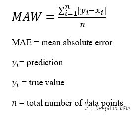
Calculate the Patch for each data point (i), and select Mae (Mean-Absolute-ERROR) as the loss function of the main sequence and reconstruction sequence.

This is the overall structure

The following is the code implementation:

DEF TRUNC_NORMAL_ (tensor, Mean = 0., STD = 1.): __call_trunc_normal_ (tensor, mean = mean, sTD = std, a = -std, b = std) Def UNSHuffle (shuffled_tokens): DIC = for k, v, in enumerate (shuffled_tokens): > dic[v] = k unshuffle_index = [] for i in range(len(shuffled_tokens)): unshuffle_index.append(dic[i ]) return unshuffle_indexclass TSFormer(nn.Module): def __init__(self, patch_size, in_channel, out_channel , Dropout, Mask_size, Mask_ratio, L = 6, Distiment = 'Uniform', LM = -1, Selected_feature = 0, Mode = 'PRETRAIN', SpecTral = TRUE): <). ) Self.patch_size = Patch_size Self.seleted_feature = Selected_feature Self.mode Self.patch = Patch (patch_size, in_Channel, out_Channel, spectral=spectral) self.pe = PositionalEncoding(out_channel, dropout=dropout) self.mask = MaskGenerator(mask_size, mask_ratio, distribution=distribution, lm=lm) self.encoder = TransformerLayers(out_channel, L) self.decoder = TransformerLayers(out_channel, 1) self.encoder_2_decoder = nn.Linear(out_channel, out_channel ) Self.mask_token = nn.parameter (torch.zeros (1, 1, 1, out_Channel)) trunc_normal_ (self.mask_token, std = .02) If Self.spectral: Self.output_layer = nn.linear (out_Channel, int (PATCH_SIZE/2+1)*2) Else: Else: Else: ELSE: ELSE: ELSE: ELSE: ELSE: ELSE: ELSE: ELSE: ELSE: ELSE: ELSE: ELSE: ELSE: ELSE: ELSE: ELSE: ELSE: ELSE: ELSE: ELSE: ELSE: ELSE: ELSE: ELSE: ELSE: ELSE: ELSE: ELSE: ELSE: ELSE: ELSE: ELSE: ELSE: ELSE: ELSE: Else

Self.output_layer = nn.linear (out_Channel, Patch_size) Def _Forward_pretrain (input): B, B, N, c, l = input.shape # get patches and exec input embedding Patches = Self.patch (input) Patches = Patches.transpose (-1, -2) # Positional Embedding Patches = Self.pe (Patches) # Mask tokens < /code> unmasked_token_index, masked_token_index = seld.mask () ENCODER_INPUT = Patches Code> # ENCODER h = Self.encoder (enCoder_input) # ENCODER to decoder h = Selfoder_2_Decoder (h) # DECODER # h_unmasked = Self.pe (h, index = un Masked_token_index) h_unmasked = H H_MASKED = Self.pe (self.mask_token.expand (b, n, len (masked_token_index), h.shape [-1]), index = masked_token_index) h_full = torch.cat ], dim = -2) # # b, n, l/p, d h = self.decoder (h_full) # Output layer if self.Spectral: # OUTPUT = H SPEC_FEAT_H_ = SELF.OUTPUT_LAY (H) Real = SPEC_FEAT_H_ [. ..,: int (self.patch_size/2+1)] Image = SPEC_FEAT_H _ [..., int (self.patch_size/2+1):] SPEC_FEAT_H = torch.complex (real, imag) out_full = torch.fft.irfft (spiec_feat_h) Else:

Out_full = Self.output_layer (h) # Prepare Loss B, N, _, _ = Out_full.Shape Out_Masked_tokens = OUT_FULL [::, Len (unmasked_token_index) :,:] Out_Masked_tokens = Out_Masked_tokens.view (b, N, -1) .tries label_full = input.permute (0, 3, 1, 2) .Unfold (1, Self.patch_size, Self.patch_size) [::, Self. Seleted_feature,:]. Transpose (1, 2) # B, N, L/P, P label_masked_tokens = label_full [:::, masked_token_index,: contiguous () > label_masked_tokens = label_masked_tokens.View (b, n, -1) .transpose (1, 2) # Prepare plot ## Note the The output_full and label_full are not aligned. The out_full in shuffled ### therefore, unshuffle for plot unshuffled_index = unshuffle(unmasked_token_index + masked_token_index) out_full_ unshuffled = out_full[:, :, unshuffled_index, :] plot_args = plot_args['out_full_unshuffled'] = out_full_unshuffled plot_args['label_full'] = label_full plot_args['unmasked_token_index'] = unmasked_token_index plot_args['masked_token_index'] = masked_token_index return out_masked_tokens, label_masked_tokens, plot_args Def_FORWARD_BACKEND (SELF, Input):

B, N, C, L = Input.shape # get patches and exec input embedding Patches = Self.patch (input) Patches = Patches.transpose (-1, -2) # Positational Embedding Patches = Self.pe (Patches) ENCODER_INPUT = Patches # No Mask When Running The Backend. # ENCODER h = Self. ENCODER (ENCODER_INPUT) Return H Def Forward (Self, Input_data): if> Self.mode == 'PRETRAIN': Return Self._Forward_pretrain (input_data) Else: Return Self._Forward_backend (Input_data) After reading this paper, I found that this can basically be said to copy MAE, or the MAE of the time sequence. It is similar to MAE during the prediction stage. It uses the output of the encoder as a feature and provides feature data for the downstream tasks as input. If you are interested, you can read the original papers and read the code given by the paper.

References

[1] Makridakis et al., The M5 Accuracy Competition: Results, Findings and Conclusions, (2020)

[2] D. Salinas et al., Deepar: Probabilistic ForeCasting with Autoregressive Recurrent Networks, International Journal of Forecasting (2019).

[3] BORIS N. Et Al., N-Beats: Neural Basis Expans Analysis for Interpretable Time Series Forecasting, ICLR (2020)

[4] Jake Grigsby et al., Long-Range Transformers for Dynamic Spatiotemporal Forecasting,

[5] Bryan Lim et al., Temporal Fusion Transformers for Interpretable Multi-Horizon Time Series Forecasting, International Journal of ForeCasting SEPTEMEM 202020202020202020202020 place

[6] Seyed Mehran Kazemi et al., Time2vec: Learning A Vector Representation of Time, Jury 2019

[7] Pre-Training Enhanced Spatial-Temporal Graph Neural Network for Multivar ass

[8] Masked Autoencoders are scalable vision lead: Yu Tengkai

- END -