At the end of 1915, the general theory of general relativity proposed by Einstein can be considered the most beautiful theory in the entire physics. However, such a beautiful theory in physical thoughts and mathematical expressions is just a formal harmonious beauty, or is it still a true description of our objective world? This article will take the first strict solution of the theory of relativity -Swani solution as an example to quantitatively test the correctness of the general theory of relativity. Although the Swanis solution is the simplest extraordinary understanding of the broader theory of gravitational field equations (static sphere symmetrical), it accurately describes the gravitational field near the sun. Under the framework of traditional Newton's gravitational theory, the planets near the sun will move around the sun to a closed ellipse track; the light near the sun will spread along the line along the straight line. So here we hope to quantitatively look at the Swai Time and Space given by the new gravity -the theory of general relativity (a gravitational field near the sun), what kind of motion trajectory of planets and light will show Different conclusions of gravity theory, how these conclusions are proven one by one by accurate astronomical observation.
1 Starcas Specifications -The Static Ball Symmetry of Einstein Formula
First consider the straight time and space described by the narrowing theory. Due to the gravitational field problem that is about to deal with the symmetrical distribution of the ball (such as the gravitational field generated by the star sun), we can systematically control the < /g> The form under the coordinate system is:
/g> < /g> < /g> < /g> < /g> < /g> < /g> < /g> /g> Now consider the gravitational field of the ball symmetrical distribution generated by a ball symmetrical substance (such as a gravitational field generated by a star located near the coordinate origin). According to the Birkhoff theorem, the degree of rules at this time must be static, that is, the amount of all degrees does not have time dependence. Inference the formal form at this time is:
/g> < /g> < /g> < /g> < /g> < /g> < /g> < g data-mml-node = "mi" /> < /g> < /g> < /g> < /g> < /g> < /g> This is a static spherical symmetry, also known as "Swroke =" CurrentColor "Fill =" Currentcolor "Stroke-Width =" 0 0 0 0 0 -1 0) "> , the score needs to be degraded to the form of Mincofski for the level and space. At the same time, it is noted that the formal parameters in the rules here have no special physical significance. This is just to facilitate the calculation and curvature after the convenience, because the calculations of the two involve the guidance of the degree of rules, and it is the simplest to find the guidance of the index function. Now in the form of rules, we can first contact it according to it, that is, the Christopofir symbol:
< /g> < /g> < /g> < /g> < /g> < /g> < /g> < /g> < g data-mml-node = "mi" /> < /g> < /g> /> /> < /g> < /g> < /g> > "> g> After some complicated calculations, we finally get the following 9 independent non -zero non -zero contact factor:
-Node = "math"> < /g> g data-mml-node = "texatom" transform = "translate (625,
413) Scale (0.707) "Data-MJX-TexClass =" Ord "> < /g> < /> < g data-mml-node = "mo" transform = "translate (583, 413) scale (0.707" "/> < /g> < /g> < /g> < /g> < /g> < /g> < /g> < /g> < /g> < /g> < g data-mml-node = "mi" /> < /g> < /g> < /g> < /G> < /> g data-mml-node = "mi" transform = "translate (7195.3, 0)"/> < /g> < /g> < /g> < /g> < /g> < /g> < /g> < /g> < /g> < /g> < /g> < /g> < /g> /g> Because of contacting There are also some non -independent non -zero -link coefficients that are not listed separately above. Readers can easily make up for the other 4 non -zero contact factor through the exchange symmetry of this lower bid, that is,:
< /g> < g data-mml-node = "mo" transform = "translate (1659.9, 0)" /> < /g> < /g> < /g> < /g> < /g> < /g> < /g> < /g> It can be found that only 13 of the original 64 contact factor! Now we can use them to calculate Riemann's tension:
< /g> < /g> < /g> < /g> < /g> < / g> < /g> < g data-mml-node = "mi" /> < /g> < /g> < /g> < /g> < /g> < /g> After some complicated calculations, we finally get the following 6 independent non -zero Riemann rates:
< /g> < g data-mml-node = "mi" /> /g> < /g> < /g> < /g> < /g> < /g> < /g> < g data-mml-node = "mn" /> < /g> < /g> < /g> < /g> < /g> < /g> < /g> < g data-mml-node = "mtd" /> g data-mml-node = "texatom" transform = "translate (759, 413) scale (0.707)" data-mjx-texclass = "order"> < /g. > < /g> < /g> < /g> < /G> < /g> < /g> < /g> < /g> < /g> < /g> < /g> /g> Readers are easy The weight of the non -zero Riman rate is replenished, that is,:
< /g> < /g> < /g> < /g> < /g> < /g> < /g> < /g> < /g> < /g> < /g> < /g> < /g> < /g> < /g> < /g> < /g> g data-mml-node = "mo" transform = "translate (2623.3, 0)" /> < /g> < /g> < /g> < /g> < /g> < /g> < /g> < /g> < /g> < /g> < /g> < /g> < /g> g data-mml-node = "mi" transform = "translate (2197, 0)" /> < /g> < /g> /g> < g data-mml-node = "mtd" /> g data-mml-node = "texatom" transform = "translate (759, 413) scale (0.707)" data-mjx-texclass = "order"> < /g. > /> < /g> < /g> < /g> < /g> < /g> < /g> < /g> < /g> < /g> < /g> < /g> < /g> /g> < /g> < /g> < /g> < /g> < /g> < /g> < /g> < /g> /g> < /g> < /g> < /g> < /g> < /G> < /g> > < /g> < /g> < /g> < /g> < /g> < /g> < /g> < /g> < /> < /> < /> < /> < /> < /> < /> < />g data-mml-node = "mn" transform = "translate (8874.6, 0)" />
It can be found that only 12 of the 256 Riemann ratio (with 4 indicators) are not zero! Now we can shrink them into Richter with only 2 indicators. "> < /g> < /g> /g> (Rich can be regarded as some kind of average of Riemann's tune, it is exactly what I really need to use in Einstein's gravitational field. The amount of curvature). Ricci originally had 16 components, but because of the high symmetry of the original regulation, it can be found that the Riemann ratio of Riemann will only get the following 4 Ricci tensor. The weight. They happen to be four diagonal elements that should be matrix (note: And not independent):
< /g> < /g> < /> < g data-mml-node = "texatom" transform = "translate (466, 413) scale (0.707)" data-mjx-texclass = "order"> < g data-mml-node = "mo" transform = "translate (1776.3, 0)" /> < /g> < /g> < /g> < /g> < /g> < g data-mml-node = "mn" /> < /g> < /g> < /G> < /g> g data-mml-node = "mo" transform = "translate (8033.6, 0)" /> < /g> < /g> < /g> < /g> < /g> < /g> < /g> /> /> < /g> < /g> < /g> < /g> < /g> < /g> < /g> < /> < /> < /> < /> < /> < /> < /> < /> < /> g data-mml-node = "msubsup" transform = "translate (9033.9, 0)"> < /g> < g data-mml-node = "mn" transform = "translate (778, 0)" /> < g data-mml-node = "mo" /> < /g> < /g> < /> < /> g> < /g> < /g> < /g> < /g> < /g> < /g> g data-mml-node = "texatom" transform = "translate (759, -253.5) scale (0.707)" data-mjx-texclass = "order"> < /> < /> g> < /g> < /g> < /g> < /g> < /g> < /g> < /g> < /g>/g> /g>
Since the substances (such as stars) we are considering the gravitational field are just limited to a small limited area near the original point, and the space -time area we really want to study is located outside the material (star), so at this time the ability to move at this time Tension < /g> < /g> < /g> < /g> < /g> < /g> < /g> /g> and its shrinkage and is 0. So what we want to solve is the simplest vacuum Aintein field equation < g data-mml-node = "math"> < /g> < /g> . Because the previously calculated amount of Richta is a diagonal matrix, so in order to allow Rich to meet the above vacuum Einstan field equations, all its diagonal element It must be 0. The specific expression of the diagonal element that the previously calculated Richter tensor is replaced:
< /g> < /g> < /g> < /g> < g data-mml-node = "mi" transform = "translate (244.5, -686)" /> < /g> < / g> < /g> < /g> < /g> < /g> < /g> < /g>
The above will be and adds:
< /> g> g data-mml-node = "mi" transform = "translate (389, 0)" /> < /g> < /g> Easy to solve:
CurrenTColor "Fill =" Currentcolor "Stroke-Width =" 0 "Transform =" Matrix (1 0 0-1 0) "> is the integral constant. The upper formula is substituted into the expression of Swadas, and the < g data-mml-node = "mi" /> < /g> Time (doing this does not affect all real physical observations):
/g> < /g> < /g> < /g> < g data-mml-node = "mi" /> < /g> < /g> < /g> < /g> < /g> This redefining is equivalent to making < g data-mml-node = "math"> ,代入 < /g> < /g> < /g> < /g> < /g> < /g> < /g> < /g> < /g> /g>
< /g> < /g> This is a first -order constant differential equation. The solution to the equation by separating variables is:
< /g> < /g> < /g> < /g> < /g> < /g> < /g> < /g> Among them, is the point constant The constant to be fixed. Replace the above form of solution into the expression of Swarzalan's rules:
-Node = "math"> /g> < /g> < g data-mml-node = "mn" /> < /g> < /g> < /g> < /g> < /g> < /g> < /g> < /g> < /g> < /g> < /g> < /g> < /g> < /g> < /g> g data-mml-node = "texatom" transform = "translate (4394.4, 1176.6) scale (0.707)" data-mjx-texclass = "order"> < /g> < /g> < /g> < /g> g> Easy to verify when , the rules are indeed degraded to the form of Mincovsky under the level and space. So so far we have set the mathematical form of Swadavadon through the vacuum Eintan equation. Regarding the constant of the rules and regulations It is true that we have to use the general theory of relativity-ground line equation. Our ideas are: under the limit of low -speed static weak fields, the ground line equation will degenerate to the motion equation given by Newton's second law and the laws of gravity.
On the one hand, the ground line equation will be degraded at low speed and weak fields:
< g data-mml-node = "msup"> < /g> < /g> g data-mml-node = "texatom" transform = "translate (556, 421.1) scale (0.707)" data-mjx-texclass = "order"> < /g. > < /g> < /g> < /g> < /g> < /g> < /g> g data-mml-node = "mo" transform = "translate (5837, 0)" /> < /g> < /g> < /g> < /g> < /g> < /g> < /g> < /g> < /g> < /g> /g> < /g> < /g> < /g> < /g> < /g> < /g> < /g> < /g> < /g> < /g> < /g> On the other hand, through Newton's second law and the law of gravitational gravity, you can writeout:
< g data-mml-node = "msup"> < /g> < /g> g data-mml-node = "texatom" transform = "translate (556, 421.1) scale (0.707)" data-mjx-texclass = "order"> < /g. > < /g> < /g> "> < /g> < /g> < /g> < /g> < /g> < /g> < /g> Among them "Transform =" Matrix (1 0 0-1 0 0) "> Classic Newton's gravitational momentum. Therefore, the results given by the above-mentioned ground wire equation and the results given by Newton's laws can be set. -1 0) "> .
Finally, the constant The value of The expression of the Swadisian regulatory expression is obtained by the Swadasu ruler under the natural unit:
< /g> < /g> < /g> < /g> < / data-mml-node = "mo" transform = "translate (5235.4, 0)" /> < /g> < /g> < /g> > < /g> < /g> < /g> < /g> < /g> < /g> < /g> < /g> /g> Sawasis Gravity is the Einstein gravitational field equation The first strict solution is also an extremely important solution. Its physical connotation is quite rich, and many important time and space situations can be described by it. For example, the gravitational field generated by the sun can be accurately described in Swadas. So let's study two specific circumstances below, namely: the launch of Mercury tracks under the sun and space generated by the sun and the bias of the ray of light and light across the sun.
2 Mercury's rails have advanced recently
With the form of Swanis's gauge in Section 1, we will now study the movement trajectory of the planet under the Star Time and Space generated by the Star (Sun). From The final solution of the Swadas Gulf in the final solution can be read directly. = "Matrix (1 0 0-1 0)"> and . Substitute it into < g data-mml-node = "mo" /> The contact coefficient expression that has been found is easy to get:
< /g> < /> < /> g data-mml-node = "mi" transform = "translate (5185.4, 0)" /> < /g> < /g> g data-mml-node = "msup" transform = "translate (3105.4, -793.2)"> < /g> < /g. > < /g> < /g> < /g> < /g> < /g> < /g> < /g> < /g> < /g> < /g> < /> g> < /g> < /g> < /g> < /g> < /> g data-mml-node = "mo" transform = "translate (4048.7,
0) " < /g> < /g> < /g> < /g> < /g> < /> < g data-mml-node = "texatom" transform = "translate (1228, 413) scale (0.707)" data-mjx-texclass = "order"> < /g. > < /g> < /g> < /g> < /g> "> < /g> The orbit of the planetary movement is given by the broader theory of relativity -the ground line equation is given. The lines can get the following as follows, respectively, < /g> Cable equations.
Note that there is no and dependence, Therefore, this degree has continuous time transitions and invariability and about rotation invariance. Therefore, according to the theorem of Norther, we look forward to the and Formula) Give two conservation: one is the energy , the other is the rail angular volume < /g> . About The ground wire measurement can be given a conservation (energy):
< /g> < /g> < /g> In order to facilitate the promotion of qualityless objects (light), the following analysis does not directly use
About
< /g> < / g> < /g> "> "> < /g> < /g> /g> To solve the above about The second-order constant differential division equation must first know the And . If the plane of stars and planet speed vector Zhang Cheng is the equator (XY plane), and the direction of the equatorial surface is the direction of Z, then:
< /g> < /g> < /g> < /g> < /g> "> This means that the speed and acceleration of the planet in the direction of the equatorial surface are 0. So the running track of the planet is a flat curve that falls on the equator.
About The ground wire measurement can be given a conservation : < /> /g> < /g>
In order to facilitate the direct promotion of quality planets discussed here to directly promote the movement of no quality photons in the third quarter, we have obtained from the perspective of the original regulation. -width = "0" transform = "matrix (1 0 0-1 0)"> < /g> differential equation. Considering the original Swadalan's rules:
-Node = "math"> /g> < /g> < /g> < /g> < /g> < /g> g data-mml-node = "mi" transform = "translate (1163,
-686) " /> < /g> < /g> < /g> < /g> < /g> < /g> < /g> < /g> < /g> < /g> g data-mml-node = "msup" transform = "translate (29793.6, 0)"> < /g> < /g> < /g>
For the quality objects we are considering now, sometimes < /g> < /g> < /g> < /g> < /g> < /g> < /g> < /g> < /g> < /g> < /g> < /g> < /g> < /g>/g> Non -zero, so you can divide the upper sides with The result of the conservation amount given by the ground measuring line equation is substituted, and the differential division equation is obtained after simplifying and consolidating:
> < /g> < /g> < /g> < /g> /g> < /g> To the form of "always energy = kinetic energy+ potential energy", it can be obtained by the effective potential function of the quality object in the broad sense of the general theory:
< /g> < /g> < /g> < /g> "> The part of the brackets is exactly the effective potential function of the quality object in Newton's gravitational theory (the first is the classic Newton's gravitational potential, and the second item is the centrifugal energy generated by the ball coordinate system).
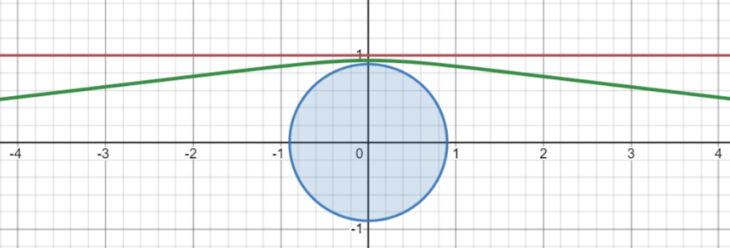
For intuitive, Figure 1 has an effective potential function that has a quality object in the general theory of Ainstein in Figure 1 and Einstein's general theory. It can be seen that the difference between the two is mainly reflected.
Figure 1 The vertical axis is effective, and the horizontal axis is a radial distance from the sun. The red line represents the effective potential function of the quality object in Newton's gravitational theory.
According to chain -type guidance rules,
-Node = "math"> > < /g> < /g> < /g> < /g> < /g> < /g> < /g> < /g> < /g> G Data-MML-Node = "Texatom" Data-MJX-TEXCLASS = "Ornsform =" Translate (2386, 0) "> < /g> < /g> < /g> < /g> < /g> < /g> < /g> < /g> < g data-mml-node = "mi" /> < /g> < /g> < /g> /g> < /g> < /g>
This < /g> The results are substituted into the previously obtained by the original norms. About slightly divided equation, and then the two ends of the prescriptions at the same time are at the same time . So the equation is simple:
< g data-mml-node = "msup"> < /g> < /g> g data-mml-node = "texatom" transform = "translate (556, 421.1) scale (0.707)" data-mjx-texclass = "order"> < /g. > < /g> < /g> < /g> /g>
The second item on the right side of the equation is easy to find the amendment item given by the general theory. The rest of the equation is exactly the same as the results given by traditional Newton's gravitational theory. The solution to the equation is < /g> , of which Stroke = "CurrenTcolor" Fill = "Currentcolor" Stroke-Width = "0" Transform = "MATRIX (1 0 0-1 0)"> Later, the slight disturbance correction of the original Newton solution. So Satisfied equation:
< g data-mml-node = "msup"> < /g> < /g> g data-mml-node = "texatom" transform = "translate (556, 421.1) scale (0.707)" data-mjx-texclass = "order"> < /g. > < /g> < /g> < /g> < /g> Easy to solve it (may be the initial phase of the orbit is 0):
0, -2711.4) "> "Transform =" Translate (220, 676) "> < / g> < /g> < /g> < /g> < /g> < /g> "> < /g>
This is exactly the cone curve equation under the polar coordinate! Among them, is the curve centrifugal rate: When Corresponding ellipse orbit, < /g> When the parabolic line orbits, < /g> < /g> G> corresponds to the bilateral track.
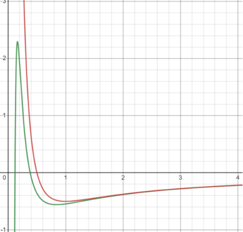
Because we are now considering a stable planet sports track, we can only take > , that is, a closed circle/ellipse orbit. This is exactly the same as the conclusion given by Newton's gravitational theory and the laws of the law of the planetary sports! Figure 2 Make a closed ellipse orbital image under the theory of Newton's gravitational theory: Figure 2 The vertical axis is Y and the horizontal axis is X. The two together became the equator where the planetary sports track was located. Blue circles located at the original point of the coordinate origin (that is, a focus point of red ellipse) represent stars, and the red line represents the closed ellipse orbit of the planet movement under Newton's gravitational theory
The following considers the micro-disturbance The equation that approximately satisfy. Note that < /g> < /g> g data-mml-node = "msub" transform = "translate (2127.6, 0)"> :
< g data-mml-node = "msup"> < /g> < /g> g data-mml-node = "texatom" transform = "translate (556, 421.1) scale (0.707)" data-mjx-texclass = "order"> < /g. > < /g> < /g> < /g> < /g> < /g> < /g> < /g> < /g> < /> g data-mml-node = "mo" transform = "translate (4082.1,
0) " /g> Simplified consolidation to get Linear constant constant differential equation:
< g data-mml-node = "msup"> < /g> < /g> g data-mml-node = "texatom" transform = "translate (556, 421.1) scale (0.707)" data-mjx-texclass = "order"> < /g. > < /g> < /g> < /g> < /g> < /g> < /g> < /g> < /g > Note that the < /g> driver It happens that the resonance frequency of the system , so there is a cumulative divergence (resonance) corresponding to the corresponding part of the driver, and This item! Because the above -mentioned differential equation has been simplified into the form of a linear equation, the solution of the above differential equation can be obtained by the superposition principle:
< /g> < /g> < /g> < g data-mml-node = "mi" /> < /g> < /g> < /g> < /g> < /g> g data-mml-node = "mi" transform = "translate (12121.8, 0)" />
So after considering the amendments to the general theory, the total solution is Newton's solution and micro-disturbance :
< /g> < /g> < /g> < /g> < g data-mml-node = "mrow" transform = "translate (528, 0)"> < /g> < /g> < /> g data-mml-node = "mo" transform = "translate (9812, 0)" /> < /g> Because the amendment given by general relativity is very small than the original Newton, so it will further and the corresponding It is similar to the form similar to the cone curve similar to the previous pole coordinates, so that Compared with the track results given by Newton's gravitational theory:
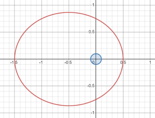
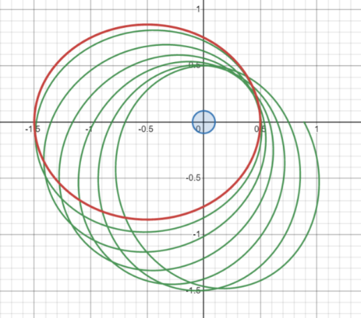
< /> < /> g data-mml-node = "mfrac" transform = "translate (1905.6, 0)"> < /g> < /g> < /g> g data-mml-node = "mo" transform = "translate (2160.8, 0)" /> < /g> < /g> < /> < /> g data-mml-node = "mrow" transform = "translate (3693.1, 0)"> < /g> < /g> < /g> < /g> /g> Because we are now considering a stable planetary sports track, we can only take < /g> < /g>. The closed ellipse orbit around the star movement and the theory of general relativity advanced the planet's ellipse orbit around the star movement. It can be seen that the orbit at this time is not a closed curve!
Figure 3 The vertical axis is Y and the horizontal axis is X. The two together became the equator where the planetary sports track was located. Blue circles located at the original point of the coordinate origin (that is, a focus point of the red ellipse) represent the stars, and the red line represents the closed ellipse orbit of the planet movement under Newton's gravitational theory; Its track has been progressing recently!
Figure 4 The vertical axis is y and the horizontal axis is X. The two together became the equator where the planetary sports track was located. Blue circles located at the original point of the coordinate origin (that is, a focus point of the red ellipse) represent the stars, and the red line represents the closed ellipse orbit of the planet movement under Newton's gravitational theory; Its track has been progressing recently!
Below we are based on < g data-mml-node = "mi" /> < /g> Specific expression quantitatively calculated the advancement of the orbital point in quantitatively Angle corner. At the nearest point of the orbit, the alarm distance from the star's radial distance < /g> so:
0) "
So the advancement angle of the near -time period of the two adjacent periods is:
< /g> < /g> < /g> < /g> < /g> The results of the corner movement of the oval orbit in Newton's gravitational theory:
/> /> /> < /g> < /g> < /g> The formula of the entrance to the above movement is obtained:
< /g> < /g> < /g> < /g> < /g> < /g> < /g> < /g> < /g> < /g> < /g> /g>
According to the above formula, it can be seen that the solar is closer to the solar ( Small) and the centrifugal rate Giver the corresponding progressive corner < /g> Value is large and easy to observe.Therefore, we choose Mercury closest to the sun as an example to calculate the corner of the Mercury track brought by the general theory effect of the general theory of relativity.The following known data about Mercury and the Suns are replaced in the formula of the above -mentioned movement angle
< /> < /> g data-mml-node = "mn" transform = "translate (1862.6, 0)" /> < /g> Find the advancement of Mercury around the sun a circlehorn:
-Node = "math"> < /g> < /g> "> < g data-mml-node = "mn" /> Because this angle is small, it is converted into a more appropriate arc second (Arcsec) As unit:
< /g> < /g> According to astronomical observations, Mercury will go around the sun every 88 days. Therefore, it is easy for us to convert the progressive angle of Mercury every century (100 years)::
< /g> < /g> < /g> < /g> < /g> < /g> < /g> < /g> So we finally draw a broad sense effect effect that will cause Mercury track to get in the past 100 years (a century) about . This angle is very small, because it means that the , or every 100,000 years (1,000 centuries) Entry appointment < g data-mml-node = "mn" /> !
Before the general theory of relativity appeared, the accurate astronomical observation results at the end of the 19th century had shown that Mercury had appointments every century. 0) "> There is an appointment with <"> G data-c = "2033"/> was clearly explained by the framework of Newton's gravitational theory (note : The track of the planet under the framework of pure Newton's gravitational theory is not strictly closed ellipse, and it actually has track progress. Because there is no real secondary problem in the real universe, so we must put other planets right right. Mercury's gravitational pulling effect is also considered. In addition, there is a self-rotating axis advancement effect caused by the difference in the age of the age), and there are about < /g> 's progressive angle cannot be explained. The theoretical calculation results of Ai Estan's general theory of relativity in the early 20th century just explained this! So theory and astronomical observation results are exactly the same! Intersection Intersection 3 When the light is plundered when the sun surface is folded
In Section 2, we have quantitatively studied the motion trajectory of the planet under the Swani time and space generated by the sun. In this section, we will study the movement trajectory when the light is across the sun. Similar to the analysis in Section 2, we should first consider the original Swadas. But for light, the line element (inherent sometimes) is constant 0. With the Sometimes the quality objects (such as planets) are sometimes different, because the inherentness of light is sometimes 0, so it cannot be used as the imitation parameter in the ground line. Essence So we need to choose other non-zero-and-free variables instead of the original and sometimes position as the imitation parameter of light. In addition, the analysis of the ground line equation of light is exactly similar to the analysis in the previous section 2. Therefore, according to the basically the same logic, it is easy to get The constant differential equation and the corresponding conservation of the concentration:
< /g> < /g> < /g> < /g> < /g> < /g> < /g> < /g> < /g> < /G> < /g> < /> < /> < /> /g> < /g> "> < /G> < /g> < /g> < /g> < /g> < /g> < /g> /g> < /g> As a result, the expression of the Swaizasi gathers at the beginning was briefly consolidated and the differential equation was obtained:
-Node = "math"> < /g> < /g> < /G> < /g> < /g> < /g> < /g> < /g> < /g> Rect width = "1339" height = "60" x = "120" y = "220" /> < /g> < /g> < /g> < /g> < /g> g>
The previous The results pushed out for comparison. It can be found that in addition to the difference in the selection of imitation parameters, the difference between the two is that the equation described above does not exist in the < /g> This classic Newton gravitational potential (because the quality of the photon is 0, there is no gravitational gravity in the form of classic Newton To. The form of an upper class to the form of "always energy = kinetic energy + potential energy" can be obtained from the valid potential function of the photon (no quality object) in the broad sense theory:
< g data-mml-node = "mi" /> < /g> < /g> < /g> The effective potential function of the photon (no quality object) in the gravity theory (because the quality of the photon is 0, so there is no classic Newton's gravitational potential at this time, only one centrifugal can be transformed into the ball coordinate system).
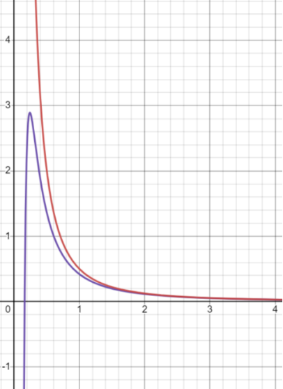
For intuitive, Figure 5 made effective potential functions in the theory of gravitational theory in Newton and Einstein's general theory in the general theory of relative theory. It can be seen that the difference between the two is mainly reflected.
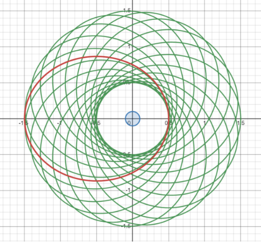
Figure 5 The vertical axis is effective, and the horizontal axis is a radial distance from the sun. The red line represents the valid potential function of the photon in Newton's gravitational theory. The purple line represents the valid potential function of the photon in the general theory of relativity
According to chain -type guidance rules,
-Node = "math"> < /g> < /g> < /G> < /g> < /g> < /g> < /g> < /g> < /g> Rect width = "1339" height = "60" x = "120" y = "220" /> < /g> < /g> < /g> < /g> data-mml-node = "mfrac" transform = "translate (736, 0)"> < /g> < /g> < /g> < /g> < /g> < /g> < /g> < /g> < /g> < /g> < /g> < /> < /> g> < /g> < /g> < /g> < /g> < /g> < /g> < /g> < /g> < /g> < /g> g data-mml-node = "mi" transform = "translate (556, 0)" /> < /g> < /g> < /g> < /g> < /g>
This < /g> The previously entered into the < / The differential equation of g> , then at both ends of the square program at the same time, Slightly divide and make < /g> . So the equation is simple:
< g data-mml-node = "msup"> < /g> < /g> g data-mml-node = "texatom" transform = "translate (556, 421.1) scale (0.707)" data-mjx-texclass = "order"> < /g. > < /g> stroke-width = "0" transform = "matrix (1 0 0-1 0)"> < /g > The . matrix (1 0 0-1 0 0) "> < /g> < /g> CurrenTColor "Fill =" CurrenTColor "Stroke-Widt h = "0" transform = "matrix (1 0 0-1 0 0)"> < g data-mml-node = "mo" /> < /g> Classic Newton's gravitational momentum.
It is easy to find the is the amendment item given by the general theory of relativity. The solution to the equation is < /g> , of which Stroke = "CurrenTcolor" Fill = "Currentcolor" Stroke-Width = "0" Transform = "MATRIX (1 0 0-1 0)"> Micro -disturbance correction of the original Newton.
So Satisfied equation:
< g data-mml-node = "msup"> < /g> < /g> g data-mml-node = "texatom" transform = "translate (556, 421.1) scale (0.707)" data-mjx-texclass = "order"> < /g. > < /g> < /g> < /g> Easy to solve (the initial phase of the orbit is 0):
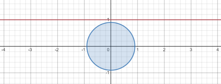
< /g> < /g> < /g> Among them, < /g> < /g> < /g>. This is exactly the (horizontal) straight -line equation under the polar coordinate! It is easy to see from the geometric relationship under the polar coordinates that the vertical distance between this horizontal straight line and the X -axis. So in Newton's gravitational theory, the light is always spread along the line! The gravitational field of the sun does not affect the transmission path of light. The root cause of this conclusion is that the classic Newton's gravitational theory assumes that the object is coupled by the only internal attribute and external gravitational field through the quality of the object. The quality of the photon is 0, so it cannot be coupled to the gravity of Newton's form, and naturally does not interact with it. Figure 6 Makes the spread of the light when the light of Newton's gravitational theory passes through the surface of the sun:
Figure 6 The vertical axis is Y and the horizontal axis is X. Together with the plane determined by the light and the sun center. The blue circle located on the coordinate original point represents the sun, and the red line represents the spread trajectory (straight line) when the light of Newton's gravitational theory passing through the surface of the sun (straight line)
The following considers the micro-disturbance The equation that approximately satisfy.Note that < /g> < /g> g data-mml-node = "msub" transform = "translate (2127.6, 0)"> :
< g data-mml-node = "msup"> < /g> < /g> g data-mml-node = "texatom" transform = "translate (556, 421.1) scale (0.707)" data-mjx-texclass = "order"> < /g. > < /g> < /g> < /g> < /g> < /g> < /g> < /> g data-mml-node = "mo" transform = "translate (1111.2, 0)" /> /g>
Because the right end of the equation does not look like There are resonance drives < /g> < /g>, and because the above differential equations have been simplified into linear equations into linear equationsThe form, so the solution of the above -mentioned differential equation can be obtained by the superposition principle:
< /g> < /g> g data-mml-node = "mn" transform = "translate (1754.3, -686)" /> > < /g> So after considering the general theory correction, the total solution width = "0" transform = "matrix (1 0 0-1 0 0)"> < /g> < /g> < /g> < /g> < /g> < /g> /g> is Newton's solution and slightly disturbing < g data-mml-node = "mi" /> :
< /g> < /g> < /g> /g> Stroke = "CurrenTcolor" Fill = "Currentcolor" Stroke-Width = "0" Transform = "Matrix (1 0 0-1 0)"> Claimed solution is:
-Node = "math"> /> < /g> < /g> < /g> Among them, the first item in the upper denomination is the lead item given by Newton's gravitational theory, and the second item is the amendment item given by the general theory. It is very small compared to the first item , That is, satisfaction: < /g> .
Figure 7 made the spread trajectory (linear) and the dissemination of the transmission of the sun under the surface of the sun and the dissemination of the sun when the light was plundered by the sun. It can be seen that the transmission path of light at this time has been biased because of the influence of the sun gravitational field!
Figure 7 The vertical axis is y and the horizontal axis is X. Together with the plane determined by the light and the sun center. The blue circle located on the coordinate original point represents the sun, and the red line represents the spread trajectory (straight line) when the light of the light of Newton's gravitational theory passing through the surface of the sun. Curve!)
Below we will be based on < /g> Specific expression of the general theory of relativity quantitatively computing the general theory of relativity quantitative theoryThe corner of the light.Because the deflection angle is related to the slope of light, you may wish to put the < /> < />g data-mml-node = "mi" transform = "translate (840, 0)" /> < /g> < /g>/g> The relationship is transformed to the right -angle coordinates to solve:
-Node = "math"> "> < /g> < /g> < /g> < /g> < /g> < /g> < /g> < /g> < /g> /g>
It can be seen from Figure 7: The green light incident incident in the upper left of the distant star on the right side was changed by the blue solar gravitational field when passing by the coordinates of the coordinates.Therefore, in order to find the corner of the entire process from infinity to infinity, we must study the approximate behavior of light in the positive and negative far away.Because the light in the infinite distance can basically be considered not to be affected by the original point of the coordinates, it can be approximately straight into a straight line.Let's set this linear equation in the following form:
< /g> < /> < /> g>
Among them, is a straight line slope.Because the amendment of the general theory of relativity is weak, the slope The mold value is small.This infinite distant distant and Formula is obtained:
< /g> < /g> < /g> < /g> < / g> When < /g>, we get the green line on the right side of the sun ( Entering light) The approximation of the infinite far away:
< /g> < /g> < /g> < /g> "> From this, the slope of the incident light can be solved, and then the angle of the incident light and the horizontal-x axis:
-Node = "math"> < /g> < /g> /> < /g> < /g> < /g> When , we get the green line (out of light) on the left side of the sun (out of light) at an infinite distance:
< /g> < /g> < /g> < /g> "> < /g> therefore can solve the slope of the light, and then obtain Angle of light and horizontal-x axis:
-Node = "math"> < /g> < /g> So the total deflection angle corresponding to the entire process from incident light to out of the outlet lightYes:
< /g> < /g> < /g> < /g> < /g> < /g> g data-mml-node = "mi" transform = "translate (1128.5, -686)" /> < /g> : When The small hour corner < /g> That is, the deflection effect is the most obvious. And The minimum can only get one solar radius Situation. Because if it is smaller than it, the light will be directly absorbed by the sun and cannot be observed. So the maximum value of the light corner is:
< /g> < /g> < /g>
< /g> < /g> can get the corner of the light when the light plunder the surface of the sun:
< g data-mml-node = "mi" /> < /g> < /g> < /g> < /g> < /g> < /g> Because this deflection angle is small, it is converted to a more suitable arc second (Arcsec):
< g data-mml-node = "mi" /> < /g> < /g> < /g> < /g> < /> < g data-mml-node = "mo" transform = "translate (4278, 413) scale (0.707)">
It can be found that this The light folding angle is very small, very small, it only has g data-mml-node = "texatom" data-mjx-texclass = "order" transform = "translate (500, 0)"> 4.87 of 10,000 per 10,000 (that is, less than data-mml-node = "math"> ! In 1919, the physicist at the University of Cambridge, Eddon, organized two observation teams to go to Polinsby and Brazil's astronomical observation to Africa. In the end, the deflection angle measured by the African Princesby team was , the Brazilian team measured < G Stroke = "CurrenTColor" Fill = "Currencolor" Stroke-Width = "0" Transform = "MATRIX (1 0 0-1 0)"> .
It can be found that the corner of the general theory of relativity theory Just fell on < /g> < /g> < /g> < /g> < /g> < /g> < /g> /g> and So theoretical and astronomical observation results are quite good! Intersection Intersection 4 conclusion
From the quantitative test of the general theory of general relativity in Section 2 and 3, it can be found that: Einstein's general theory of relativity not only has mathematical forms, but also a true description of our objective world! It is the perfect fusion of these two that has made general relativity the most successful and fascinating theory in the history of physics!
Edit: Shepherd
- END -