Look at the hydrogen atomic spectrum from three different levels

The rapid development of physics in the 20th century depends to the establishment and development of quantum mechanics. One of the important driving drivers for promoting the birth of quantum mechanics is to explain the atomic spectrum. This article will take the simplest atomic system (that is, "hydrogen atom", which is a neutral atom with only one extra -nuclear electron, but has a very important position in quantum mechanics) as an example. In accordance with the sequence of historical development, from Bohr, respectively, respectively from Bohr respectively. The old quantum theory (Bohr's orbital model), Xue Dingzhang's non -relative theoretical quantum mechanics (volatility), and Dirac's relative theoretical quantum mechanics, these three different levels of the scores of hydrogen atoms. At the first level, Bohr's experiment from the spectrum line guessed that the orbital angle of the electrons in the hydrogen atom was based on a certain physical constant as the minimum unit. Some very simple classic Newtonian mechanics and electrical derivation gives the phenomenon formula of hydrogen atomic spectrum; the latter two levels are based on the framework of quantum mechanics, and directly through the first principle of the first principle A spectrum of hydrogen atoms is given. The difference is just that the previous one did not consider the theory of narrow sense, and the latter considers the amendment of the theory of relativity. In the end, we were surprised to discover that the results of the can be strictly derived from the primary principles through complex mathematical procedures. Although from the perspective of the current orthodox quantum mechanics, many concepts in the Bohr's orbital model are problematic, but Bohr has a key physical image of the hydrogen atom through the "problematic" model of his semi -classic and semi -quantum "problematic" model. Guess it is extremely accurate! Therefore, here must admire Bohr's strong physical intuition and insight.

1 In the semi -classic and semi -quantum Bohr orbit model, see the hydrogen atomic can spect the old quantum theory

Consider the electronic wounds in the hydrogen atom to do a circular motion. The circular radius is . According to the classic Newton's second law and the form of Curon, you can give:

< g data-mml-node = "mi" /> < /g> < /g> < /g> < /g> < /g> < /g> /g> < /g> < /g>

Then Bohr boldly assumes that the electrons' orbit angle volume A physical constant (Now called "Kyathering Planck constant") as the minimum unit quantization:

< /g> The above two forms can find the speed of the electronic surround nucleus:

-Node = "math"> /g> < /g> < / G> So that the electron surround radius is:

Electronic energy is always the sum of kinetic energy and Kulun's potential energy The

-Node = "math"> < /g> data-mml-node = "mi" transform = "translate (3037.6, 0)" /> < /g> /g> < /g> Among them, < /g> < /g> << g data-mml-node = "texatom" data-mjx-texclass = "order" transform = "translate (6171.7, 0)"> < /g> Call "fine structure constant". For hydrogen atoms, the atomic nucleus is charged with a unit, that is, , so the hydrogen atomic spectrum is:

< /g> < /g> < /> < /> < /> < /> < /> < /> g data-mml-node = "mo" transform = "translate (2545.8, 0)" /> So the frequency of emission/absorbing light when electrons are transmitted at different levels of hydrogen atoms (corresponding to the physical observation volume of the spectral line, the amount of observation of the spectrum line can be volume,)),:,

< /g> < /g> /> < /g> < /g> < /g> < /g> < /g> < /g> In addition, you can also get The rail radius of the hydrogen atomic base state electron is:

< /g> < /g> < /> < /> < /> < /> < /> < /> < /> < /> g data-mml-node = "mfrac" transform = "translate (2266.1, 0)">

This radius It is also called "the first Bohr radius". It is the rail radius of the most recent energy electronic nuclear movement from the atomic nucleus. 2 Look at the hydrogen atomic can not have a relative theoretical quantum mechanics in Xue Ding's square

Considering the framework of non -relative quantum mechanics, at the ball symmetrical Kulun potential (central force field) < /g> < /g> The wave function described by the hydrogen atomic state < /g> < /g> The fixed state Xue Dingzhang equation (the time part is only a pure phase factor):

< g data-mml-node = "mn" /> < /g> < /g> g data-mml-node = "texatom" transform = "translate (466, 363) scale (0.707)" data-mjx-texclass = "order"> < /g. > < /g> < /g> The system potential field has the symmetrical characteristics of the ball, so it is used to solve the above Xue Dingzhang equation in the form of a ball coordinate table. Open the Laplas operator in Hamilton in the ball coordinate system:

< g data-mml-node = "msup" transform = "translate (826.3, 676)"> g data-mml-node = "msup" transform = "translate (1378, 0)"> < /g> < /g> < /g> < /g> < /g> < /g> < /g> "> < /g> < /g> g data-mml-node = "mi" transform = "translate (2130.7, 0)" /> < /g> < /g> < /g> < /g> < /g> < /g> < /g> < /g> < /g> < /g> < /g> < /g> < /g> < /g> This is a

The separation variable method < /g> < /g> Disassemble the above partial differential equation into 3 constant differential equations:

-Node = "math"> < /g> < /g> < /g> < /g> < /g> < /g> < /g> < /> < /> g> < /g> < /g> < /g> < g data-mml-node = "mi" transform = "translate (500, 0)" /> < /g> < g data-mml-node = "mi" /> < /g> < /g> < /g> g data-mml-node = "mo" transform = "translate (10354, 0)" /> < /g> < /> g data-mml-node = "mo" transform = "translate (19964.3, 0)" /> < /g> < /g> /g> < /G> < /g> "> < /g> < /g> < /g> < /g> < /> g> < /g> < /G> < /g> < /g> < /g> < /g> < /g> < /g> < /g> < /g> < /g> < /g> < /g> g data-mml-node = "mrow" transform = "translate (3768.7, 0)"> < /g> < /g> < /g> < /g> < /g> < /g> < /g> < /g> < /g> < /g> < /g>

Considering that The one-time and periodicity of the ), it is easy to solve:

< /> < /> g data-mml-node = "msup" transform = "translate (1863.6, 0)"> "> < /g> < /g> < /g> < /g>

The above < /g> Substituted about Formula and define variables < /g>. So the original about < The equation of g data-mml-node = "mi"/> can be converted to Formula:

< /g> < /g> < /g> < /g> < /g> < /g> < /g> < /g> < /g> < /g> < /g> < /g> < /g> < /g> < /g> /g> < /g>

When , that is, when the angular volume is projected in the z direction, the = "Currentcolor" Fill = "Currentcolor" Stroke-Width = "0" Transform = "Matrix (1 0 0-1 0)">

/g> Instead of equation < /g>:

< /g> < /g> < /g> < /g> < /g> < /g> < /g> < /g> < /g> < /g> < /g> /> /> < /g> < /g> < /g> < /g> < /g> Because it is a constant formula, each < /g> The coefficients must be 0. RentColor "stroke-width =" 0 "transform =" matrix (1 0 0-1 0) "> Between the recursive relationship:

< /g> < /g> < /g> < /g> < /g> < /g> < /g> < /g> The subscription cannot be less than 0, so the above -mentioned recursive relationship is only applicable to < g data-mml-node = "math"> .

The "> < /g> You can directly set < /g> .

Replace the recursive relationship and initial conditions of the coefficient into level expression formula is obtained:

< /g> < /g> < /g> < /g> < /g> < /g> < /g> < /g> < /g> g data-mml-node = "mi" /> < /g> < /g> < /g> > < /g> < /g> < /g> < /g> < /g> 0 "transform =" matrix (1 0 0-1 0) "> , Grade number disintegration and divergence, so you must choose Let the above -mentioned infinite number interruption into polynomial to ensure the physical understanding of convergence. It is easy to see that the method of picking at this time must be:

< /g>

Among them, called "angle quantum number".When When taking the general integer, that is, when the angular volume is projected in the z direction, the < /g> < /g> < /g> < /g> < /g> < /g>/g> Write into the following level of number:

< /g> < /g> < /g> < /g> < /g> data-mml-node = "mn" transform = "translate (458, 0)" /> < /g> < /g> < /g> < /g> The initial to The equation is obtained:

< /g> < /g> < /g> < /g> < /g> < /g> < /g> < /g> g data-mml-node = "mrow" transform = "translate (16884.1, 0)"> < /g> < /g> < /g> < /g> < /g> < /> < /> g> < /g> /g> < /g> < /g> < /g>

Because it is a constant formula, each < /g> < /g> < / G> the previous coefficient must be 0. Therefore, it is easy to get the expansion coefficient

< /g> < /g> < /g> < /g> < /g> < /g> < /g> < /g> < /g> < /g> < /g> < /g> /g> Note: In order to test the correctness, it is easy to find < /g> The above -mentioned recurrence relationship is indeed degraded to the situation where the original angle momentum is projected in the Z direction.

Because the sub -bidding coefficient of the level cannot be less than 0, the above -mentioned recursive relationship is only applicable to .

The "> and < /g> You can directly set < /g> .

Then, with the previous < g data-mml-node = "mi" /> The calculation of the same logic, that is, for the general , The level of the level of dispersion and divergence of non-physical, so you must choose the For polynomial to ensure the physical understanding of convergence. It is easy to see at this time The method of picking must be:

"> < /g> < /g> < /g> "Fill =" Currentcolor "Stroke -Width =" 0 "Transform =" Matrix (1 0 0-1 0) "> The previous < /g> Completely consistent.

The definition of g data-mml-node = "mo" transform = "translate (4921, 0)" />

So The range is , that is, for a fixed < /g>

You can have Total The spatial orientation of different methods/different Z-direction projection (where ". The name is because the number of magnetic quantums . Finally, < g data-mml-node = "mi" /> Interests into the beginning of the radial Formula is obtained:

< /g> < /g> < /g> < /g> < /g> < g data-mml-node = "mn"/> < /> < / g> < /g> < /g> < /g> < /g> < / g> < /g> < /g> < G DAT a-mml-node = "mi" transform = "translate (736, 0)" /> < /g> < /g> Note: The following is the following is: below Another method of getting the radial equation with an equivalent price.

Note that the Laplas operator in Hamilton volume of Xue Dingzhang's equations contains the total orbital angle of the corner of the rail angle, and then the total rail corner volume of the square is used. The conclusion, so we have:

< /g> < /> < /> g> < g data-mml-node = "msub"> < /g> "> -mml-node = "mn" transform = "translate (901.8, 676)" /> < /g> < /g> < g data-mml-node = "mi" transform = "translate (454.5, 676)" /> < /g> < /g> < /g> < /g> < /g> < /g> < g data-mml-node = "mi" /> < /g> < /g> < /g> < /g>

< /g> < /g> < /g> < /g> < /g> < /g> < /g> < /g> < /g>

< /g> < /g> < /g> < /g> < /g> < /g> < g data-mml-node = "mi" /> < /g> < /g> < /g> < /g> < /g> < /g> < /g> /g> < /g> < /g>

< /g> < /g> < /g> < /g> < /g> < /g> < /g> < /g> < /g> < /g> < / g> < /g> < /g> < G DAT a-mml-node = "mi" transform = "translate (736, 0)" /> < /g> < /g> The radial equation obtained by the method method is completely consistent with the radial equation obtained by the previous method. But in this way, the radial equation will be faster.

Because the hydrogen atomic problem has spherical symmetry (that is, the rotation of three -dimensional space), there is always a chance to conservation on the sphere.

Because the surface area of ​​the three-dimensional space is proportional to the , so the probability of the unit area must be proportional to , so the radial wave function must be proportional to the < g data-mml-node = "math"> ,

So you can set the to get /g> equation:

< /g> "> < /g> > < /g> < /g> < /g> < /> g data-mml-node = "mo" transform = "translate (909.2, 0)" /> < g data-mml-node = "mi" /> < /g>

First look at the gets close behavior. When , the above equation degenerates into a free situation at an infinite distance. When , is a shock solution, the corresponding radial wave function The requirements that do not meet the bondage solution that can be accumulated (at this time the solution should be scattered), So

When , Take the index attenuation and solution (the index rising to solve the non-physical house), the corresponding < /g> < /g> Corresponding restraint:

< /g> < /g> /g>

When , about solution:

or < /g> < /g> < /g> < /g> Or /g>

The first < g data-mml-node = "mi" /> The solution is because , so it is not a physical solution.

So you can only take < g data-mml-node = "mi" /> or . So according to In < /g> The behavior can < The general form of g data-mml-node = "mi"/> is set to:

< /g> < /g> < g data-mml-node = "mo" /> < /g> < /g> < /g> < /g> /> < g transform = "translate (1020, 0)"> < /g> < /g> < /g> < /g> g data-mml-node = "mo" transform = "translate (521, 0)" /> < /g> < /g> g data-mml-node = "texatom" transform = "translate (368.4, 1150) scale (0.707)" data-mjx-texclass = "order"> < /g. > < /g> /g> Integrate the number of unsubscribes to the original and unsubscribed. Formula is obtained:

< /g> < /g> /g> < /g> < /g> < /g> < /g> g data-mml-node = "mo" transform = "translate (1939, 0)" /> < /g> < /g> /g> < /g> < /g> < /g> < /g> < /g> < /g> < /g> < /g> < /g> < g data-mml-node = "mo" /> < /g> < /g> < g data-mml-node = "mo" /> < /g> < /g> < /g> < /g> g data-mml-node = "msub" transform = "translate (29019.5, 0)"> < /g> < /g> g>

Because it is a constant formula, each < /g> < /g> < / G> the previous coefficient must be 0. Therefore, it is easy to get the expansion coefficient

< /g> < /g> < /g> < /g> < /g> < /g> < /g> < /g>

You can directly determine < /g> < /g> or < /g> < /g>. For simplicity, take .

For ordinary value, Properly select allows infinite number to interrupt the polynomial to ensure the physical understanding of convergence.It is easy to see at this time The method of picking must be satisfied:

< /g> < /g> < /g> The

< /g> The definition of < /g> Main quantity number.

So for a fixed , the number of angle quantum G Stroke = "CurrenTColor" Fill = "Currencolor" Stroke-Width = "0" Transform = "MATRIX (1 0 0-1 0)"> "> . For the situation of hydrogen atoms, , so we come to the score in the special case of hydrogen atom::

< /g> < /g> < /> < /> < /> < /> < /> < /> g data-mml-node = "mo" transform = "translate (2545.8, 0)" /> < /g> It can be found that the conclusion given by Bohr's semi -classic and semi -quantity track model!

From the above, the expansion coefficient The recursive relationship between polynomial solution. Below we are at the hydrogen atom Situation The lowest level (base state) < /g> It corresponds to the radial position with the largest probability of electrons and the first Bohr radius .

Because the base state corresponds to < g data-mml-node = "mi" /> , so < /g> It can be seen that at this time, you can only take ,,

Corresponding to , so the radial wave function and probability are:

< /g> g data-mml-node = "texatom" data-mjx-texclass = "order" transform = "translate (738, -312.4)"> < /g> < /g> < /g> < /g> < /g> < /g> < /g> < /g> < /g> /g> < /g> < /g> < /g> < /g> < /g> < /g> < /g> < /g> < /g> < /g> < /g> < /g> < /g> /g>

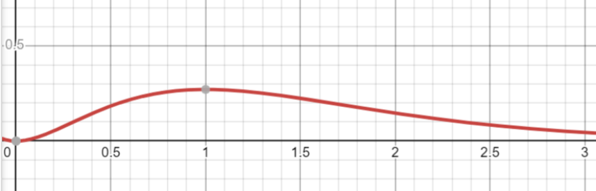
< g data-mml-node = "mrow"> < /g> < /g> < /g> < /g> g data-mml-node = "mi" transform = "translate (389, 0)" /> < /g> < /g> < /g> < /g> < /g> < /g> < /g> < /g> < /g> < /g> < /g> < /g> So the extreme point of the radial probability density function corresponds to:

< /g> < /g> < / g> < /g> < /g> Stroke = "CurrenTcolor" Fill = "Currentcolor" Stroke-Width = "0" Transform = "Matrix (1 0 0-1 0)"> or < /g> < g data-mml-node = "texatom" data-mjx-texclass = "order" transform = "translate (2804.5, 0)"> < /g> .

It is easy to see from Figure 1 below. "math"> The corresponding probability density function is very small, so it is given up; 0 "transform =" matrix (1 0 0-1 0) "> /> < /g> < /g> The corresponding probability density function is maximum.

It can be found that this < g data-mml-node = "menclose"> < g data-mml-node = "mn" transform = "translate (616.4, 413) scale (0.707" /> < /g> < /g> The radial position is just a text At the beginning of the chapter, the first Bohr radius is calculated in the semi -classic and semi -quantum Bohr's orbital model! Therefore, although the quantum mechanical effect can cause the electrons in the base state to be scattered anywhere in the whole space, the first Bohr orbit corresponds to the radial position that is most likely to discover the base state electron!

3 Look at the Dirak equation to see the hydrogen atomic can spect the relative theoretical quantum mechanics

The above is discussed under the framework of non -opposite quantum mechanics. Now considering that under the framework of relativity quantum mechanics, it is worth noting that: relativity quantum mechanics is just a transitional intermediate framework, and the self -consistent fusion of narrowing theory and quantum mechanics needs to be used. Discussion, < /g> < /g> < /g> The rotary wave function described by the electronic state below (Time part is just pure phase factor):

< /g> < /g> < /> g data-mml-node = "mi" transform = "translate (8773.9, 0)" /> < /g>

Among them, < /g> is four < /g> < /g> matrix. Select the and Dirac equation that meets the amount of rotation:

< /g> < /g> "> < /g> /g> > < /g> < /g> < /g> Among them, the Dirac Rotal Rippling Function can be decomposed into a radial wave function and an angle-to-ball harmonious function (because the system has three-dimensional space rotation, do not rotate without rotationConstruction form of degeneration):

-mml-node = "mtr" transform = "translate (0, 700)"> < /g> < g data-mml-node = "mo" transform = "translate (477, 0)" /> /> < /g> "> < /g> The following processing idea is to use the symmetrical relationship between the two rotation angles of the upper and lower rotation functions The two ends are disappeared at the same time. After some complicated operations, it can be finally simplified into a pair of a pair of radial Dirac equation (note that the test value of the radial equation corresponds to the ability spectrum). Considering that the hydrogen atom problem has spherical symmetry (that is, the rotation of three -dimensional space), so there is a total chance of conservation on the sphere.

Because the surface area of ​​the three-dimensional space is proportional to the , so the probability of the unit area must be proportional to , so the radial wave function and < /< g data-mml-node = "mo" transform = "translate (550, 0)" /> The amplitude must be proportional to

So you can set the < g data-mml-node = "mi" /> < /g> And < /g> < /g> and substituted is then obtained by the radial CurrenTColor "Stroke-Width =" 0 "Transform =" Matrix (1 0 0-1 0) "> And One -to -one -one -order coupling equation group:

< /g> /g> < G data-mml-node = "texatom" data-mjx-texclass = "order"> < /g> < g data-mml-node = "mi" transform = "translate (220, 676)" /> < /g> < /g> < /g> < /g> < g data-mml-node = "mi" /> < /g> < /g> < /g> < /g> < /g> < /g. > < /g> < /g> < /g> < g data-mml-node = "mi" transform = "translate (458,

0) " < /g> < /g> < g data-mml-node = "mi" /> Among them, is the quantum number of quantum, it is the conservation of the Dirac equation ( Corresponding to good quantum number). It replaces the position of the number of rail angular quantum quantum, because the original rail angle volume is not conserved in the Dirac equation, so it does not correspond to the number of quantum numbers.

The following is similar to the logic in the second section. By analyzing the and in < /g> < /g> The approximation of can make and The general form of solution is set separately:

/g> < /g>

-Node = "math"> < /g> < /g> < /g> < /g> < /g> < /g> < g data-mml-node = "mo" transform = "translate (10756.6, 0)" /> < /g>

The interdependence of this level of the formation into the first-order coupling equation group that was found at the beginning got a pair of labels < /g> Formula:

< /g> < /g> < g data-mml-node = "mo" transform = "translate (878, 0)" /> < /g> < /g> /g> < /g> < /g> < /g> < /> g data-mml-node = "mn" transform = "translate (3000, 0)"/> < /g> -mml-node = "mo" /> < /g> < /g> < /g> < /g> < /g> < g data-mml-node = "mfrac" transform = "translate (12023.5, 0)"> < /g> < / g> < /g> < /g>

< /g> < /g> < g data-mml-node = "mo" transform = "translate (878, 0)" /> < /g> < /g> /g> < /g> < /g> < /g> < /> g data-mml-node = "mn" transform = "translate (3000, 0)"/> < /g> -mml-node = "mo" /> < /g> < /g> < /g> < /g> < /g> < g data-mml-node = "mfrac" transform = "translate (11923.5, 0)"> < /g> < / g> < /g> < /g> Since it is a constant formula, each The coefficients must be 0.A set of recursive relationships here:

-Node = "math"> < /g> < g data-mml-node = "mi" /> < /g> < /g> < /g> < /g> < /g> < /g> g> < /g> < /g>

-Node = "math"> < /g> < g data-mml-node = "mi" /> < /g> < /g> < /g> < /g> < /g> < /g> g> < /g> < /g> For the general value, 和 The number of levels and dispersion and divergence is non -physics, so the makes the infinite number interrupt the polynomial to ensure the physical understanding of convergence.

In other words, there must be a non-negative integer , so that < /g> < /g> , but < /g> < /g> < /g>

Instead of the above-mentioned recursive relationship (take ) Get:

-Node = "math"> < /g> < /g> < /g>

-Node = "math"> < /g> < /g> < /g> It is easy to find that the above two equations are not independent. Therefore, you can get and

< /g> < /g> < /g> < /g> < /g> < /g >

Take Get a set of recursive relationships and determine through this set of recursive relationships to determine the :

-Node = "math"> < /g> < /g> < /> g data-mml-node = "mo" transform = "translate (4863.9, 0)" /> < /g> < /g> < /g> < /g> < /g> < /g> < /g> < /g> < /g> < /g> g data-mml-node = "msub" transform = "translate (16374.3, 0)"> < /g> < /g> < g data-mml-node = "mn"/> < /g> < /g> < /g>

-Node = "math"> < /g> < /g> < /> g data-mml-node = "mo" transform = "translate (4863.9, 0)" /> < /g> < /g> < /g> < /g> < /g> < /g> < /g> < /g> < /g> < /g> g data-mml-node = "msub" transform = "translate (16574.3, 0)"> < /g> < /g> < g data-mml-node = "mn"/> < /g> < /g> < /g> The and The proportional relationship.

At the same time, in order to eliminate the < g data-mml-node = "msub"> and , take the < /> < g data-mml-node = "mn" transform = "translate (433, 363) scale (0.707" " /> < /g> ,,

The two ends of the second equation are also multiplied by , and then the two forms are added:

< /g> < /g> < g data-mml-node = "mi" transform = "translate (389, 0)" /> < /g> < /g> < /g> < g data-mml-node = "mn"/> < /g> < /g> < /g> < /g> < /g> < /g> g data-mml-node = "texatom" transform = "translate (429, -150) scale (0.707)" data-mjx-texclass = "order"> < /> g> < /g> Because of us At the beginning, it was assumed that < /g> , In order to make the above equation, the formula in the bracket must be 0. In this way, we successfully eliminate all the recursive coefficients appearing in the recursive relationship equation, so as to obtain an energy constraint equation. The previous The definition of the definition substitution can be obtained:

< g data-mml-node = "mi" /> /g> < /g> < /g> < /> g data-mml-node = "mi" transform = "translate (6086.3, 0)" /> < /g> < g data-mml-node = "mi" /> < /g> < /g> < /g> < /g> < /g> < /g> < /g> /g> < /g> < /g> < /g> < /> < /> g data-mml-node = "msup" transform = "translate (2864.4, 0)"> < /g> < /g> < /g>

-Node = "math"> g data-mml-node = "msup" transform = "translate (3034.1 , 0) "> < /> < /> g data-mml-node = "mo" transform = "translate (3065.4, 0)" /> < /g> < /g> "> < /g> < /g> Last substitution < /g> The definition of solution can be solved is:

< /g> < /g> <"> <"> < g data-mml-node = "mrow"> < /g> < /g> < /g> < /g> < /g> < /g> < /g> < G transform = "Translate (1020, 0)"> < /g> < /g> < g data-mml-node = "mn"/> < /g> < /> g> < /g> < /g> < /g> < /g>

Among them, < /g> < /g> < g data-mml-node = "texatom" data-mjx-texclass = "order" transform = "translate (2843.1, 0)"> < /g> < /g> 是精细结构常数（注意这个 and the previously defined is not the same ). It is easy to find that there is a positive and negative and negative symmetry here. The positive spectrum corresponds to the energy spectrum of normal electrons, and the negative spectrum corresponds to the energy spectrum of anti -particles (anti -electron/positive electrons). In order to compare with the situation of non -opposite theory before, we will not consider the energy spectrum and energy stimulus mode of anti -particle here for the time being.

For the situation of hydrogen atoms, , so < /> < /> g data-mml-node = "texatom" data-mjx-texclass = "order" transform = "translate (3419.6, 0)"> < /g> < /g> It can be regarded as a micro -interference coupling parameter of the system. So press < /g> (~ fine structure ~ fine structure Normal) Miqi Taylor Expand (small expansion):

< /g> < /g> < /g> < /g> < /g> < /g> < g data-mml-node = "mn"/> < /g> < /g> /> < /g> < /g> < /g> < /g> < /> < g data-mml-node = "mi" transform = "translate (389, 0)" />

The definition of < /> /g> The main quantum number. It is easy to find the first energy. Its role is only to make the overall upward translation of the energy of the system, which does not affect the specific spectrum structure and related dynamic behaviors, so it has nothing to do with our current discussion. After the zero point can be deducted, you can find that the most important structure of the energy spectrum is determined by the second item of the previous formula (because is a small amount):

-Node = "math"> < /g> < /g> < /g> < /< /> g data-mml-node = "texatom" transform = "translate (466, 363) scale (0.707)" data-mjx-texclass = "order"> < /g. > < /g> For hydrogen atoms, , so the main structure of hydrogen atomic spectrum is:

< /g> < /g> < /> < /> < /> < /> < /> < /> g data-mml-node = "mo" transform = "translate (2545.8, 0)" /> < /g> It can be found that this can be found that the conclusion given by Bohr's semi -classic and semi -quantity rail model! And this result is also the result. The conclusions of the description of the description of the Xue Dingli Formula of the hydrogen atom are consistent!

However, unlike Xue Ding's square equations: Due to the narrowing theory effect, the Dirac equation also gives Boer's high -level correction! This high -level correction can be seen from the third item of the level of the scores above. This correction item will cause a weak split to the original Boer energy level, which corresponds to the fine structure of hydrogen atomic energy spectrum! This fine structure cannot be given from the non -relative theory of hydrogen atom Xue Ding.

Edit: Shepherd

- END -