The Vlowup function is not available, no wonder you always work overtime

Today, I plan to write a graphic collection of a common function class, so that everyone can find or learn some common functions in the work. Today is the first. Let's learn a well -known Excel function -vlookup. It is a must -have One of the functions, let's learn this function below

1. The role and parameters of vlookup

Vlowup: A vertical search function in Excel. The word vertical is the key. It indicates the function of the function and is based on the data query. Corresponding to it is the HLOOKUP function, it is a vertical search function, which is exactly the same as VLOOKUP

Grammar: = vlookup (search value, find the area, the number of columns, matching methods where the result is located)

First parameter: Find the value, want to query the second parameter based on that data: find the area, to find data in that data area to query the third parameter: the number of columns where the result is, the result we want to find is the second parameter Several columns of the fourth parameter: matching method, there are 2 inquiries and matching methods, accurate matching and approximate matching settings to 0 or false indicate accurate matching, the function will not find the result, the function will return to#n/a, this is the most commonly used The matching method is generally selected for accurate matching

Set to 1 or true represents approximate matching. If the result is not found, Vlowup will return the maximum value of less than the search value.

The above is the parameter and role of vlookup. Then we have used several examples to understand how it uses its use

Example demonstration

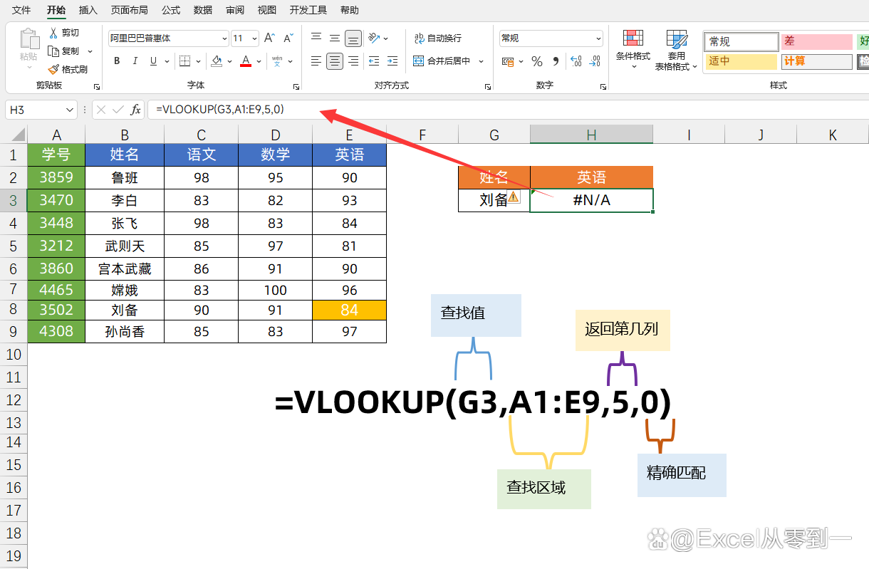
As shown below, we want to find [Liu Bei's English results]

The formula is: = vlookup (G3, A1: E9,5,0)

The first parameter: G3, the search value, it is the cell location where [Liu Bei] is located

Second parameter: A1: E9, the data to find, it means that data query is required in this area

Third parameter: We need to count, the result we need to find is the first column of the second parameter. In this example, [English score] is in the 5th column, so it is set to 5

Fourth parameter: 0, indicating accurate matching.

Third, precautions

Using the vlookup function, we need to pay attention to 2 points, which is why many people use the VLOOKUP function to make an error

1. The search value must be in the first column of the data area

As shown in the figure below, find [Liu Bei's English results]. The formula is still the same formula. It is only set to the first column in the data source [Xue Number], and the function returns the error value of#n/a. The characteristics of the Vlowup function.

When we use VLOOKUP for data query, the search value must be in the first column of the search area, otherwise the function will return [error value]. This is a hard condition that cannot be changed!

For such problems, the solution is very simple. I just need to paste the search value to the front of the data source, and then perform the data query. After the query is completed, it can be hidden. ] Solution

Formula: = vlookup (H3, A1: F9,6,0)

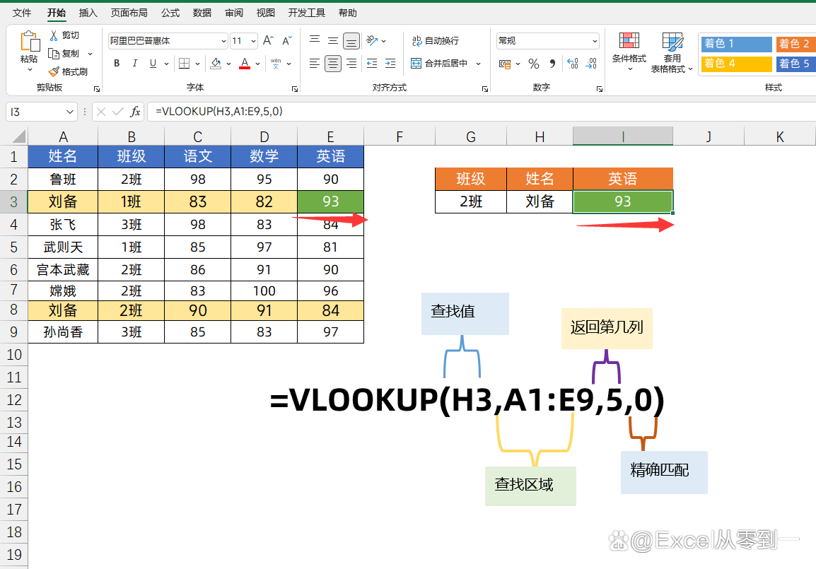
2. In encountering the duplicate value, you can only return the first result to find

This feature not only refers to VlowUp, all the [search functions] in Excel are like this. If you encounter duplication, you can only return the result of the first one

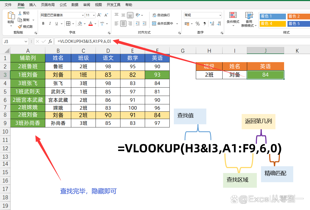
As shown in the figure below, we want to find the English results of [Class 2 Liu Bei]. Now there is a re -name in [Liu Bei] in the data source. If you still use the name [Liu Bei] to query the data, the result is [Class 1 Liu Bei English results] Because the query direction of the function is from bottom to top, Liu Bei 1 Liu Bei is in the first position, so this result will be returned. If you want to solve such a problem, we must add a condition to the only one to find the target of the finding value in order to find the grades of Liu Bei in 2 class. This is the so -called multi -condition query

Here we use connection symbols in the data source, connect the class with the name together, and build a auxiliary column. This auxiliary column is the only one, so it can be queried according to the data after the merger.

Auxiliary column formula: = C2 & B2

The formula is: = vlookup (H3 & i3, A1: F9,6,0)

The first parameter: H3 & i3, connect the class with the name together the second parameter: A1: F9, the finding data area third parameter: 6, the result ranks fourth parameter: 0, accurate matching accurate matching

The above is the 2nd precautions of the Vlowup function. We know that there are so much about VLOOKUP. After all, it is nearly 40 years old. Now the more powerful XLookup and Filter functions have been here for a long time. For complex issues, we can fully problems. Use these 2 functions, will be mentioned in the future

I am Excel from zero to one, follow me, and continue to share more Excel skills

Learn Excel from zero, improve efficiency and do not work overtime

Here ↓↓

- END -