Causal inference Introduction: Why do causal inferences need causality?

Source: Paperweekly

This article is about 13200 words. It is recommended to read 15+ minutes

This article is a Chinese note at the causal inferring course of causal inferring course introduced by Brady Neal.

This article is a Chinese note at the causal inferring course of the causal inference course introduced by Brady Neal.

Course homepage:

https://www.bradyneal.com/causal-inference-course

Lecture note:

https://www.bradyneal.com/intropUction_to_CAUSAL_INCERENCE-DEC17_2020-sal.pdf

Course video:

https://www.youtube.com/playList?List=ploazktcs0rzb6bb9l508cyj1z- u9iwka0

1. Why do causal inferences need causality

1.1 Simpson paradox

First of all, consider an example that is very related to the actual situation: for some kind of new crown virus COVID-27, assuming there are two therapies: scheme A and solution B, B, more scarce than A (more consumed medical resources), so it is currently accepting acceptance The proportion of patients A patients to the patients B is about 73%/27%. Imagine that you are an expert and need to choose one of the therapies, and this country can only choose this therapy. Then the question comes, how can you choose as little as possible to reduce death?

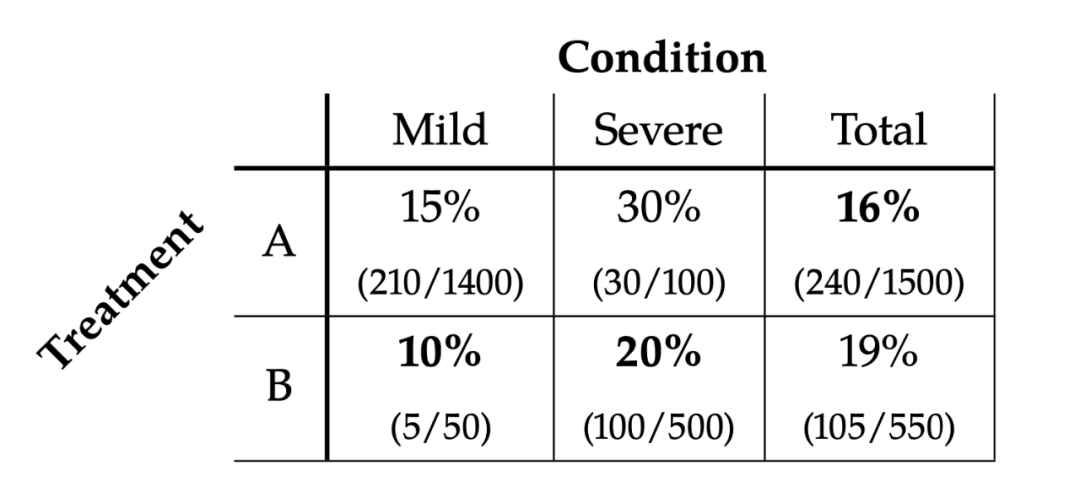
Table 1.1

Suppose you have a percentage data about the person who dies in Covid-27 (Table 1). The treatment they received was related to the severity of the condition. Mild represents mildness and Severe said torture. In Table 1, a total of 16% of the people who accept the scheme died, and the mortality rate of accepting B is 19%. We may think that the mortality rate of the treatment plan B is cheaper than cheap treatment scheme A. To be higher, isn't this outrageous? However, when we look at mild and severe (Mild column and Severe column), the situation is indeed the opposite. In these two cases, the mortality of accepting B is lower than A.

At this time, the magical paradox appeared. From the perspective of the global perspective, we are more inclined to choose A scheme, because 16%<19%. However, from the perspective of Mild and Severe, we are more inclined to plan B, because 10%<15%, 20%<30%. At this time, you gave a conclusion as an expert: "If you can judge whether the patient is mild or severe, use the plan B. If you can't judge, use the plan A". At this time, it is estimated that you have been scolded by the people as a brick home.

The key factor that leads to the occurrence of Simpson's paradox is the non -uniformity of each category. One of the 1,400 people who received A treatment of A were mild, and 500 of the 550 people received B were seriously ill. Because the mild person with a mild person is less likely to die, this means that the total mortality rate of people who receive the treatment A is less than half of the people with mild disease and severe condition. The situation of treatment B is the opposite, which leads to 16%<19%of Total.

In fact, scheme A or scheme B may be the correct answer, which depends on the causal structure of the data. In other words, causality is the key to solving Simpson's paradox. Below, we will first give me a scheme A, when should it be biased to the solution B. The theoretical explanation will be put in the back.

SCENARIO1

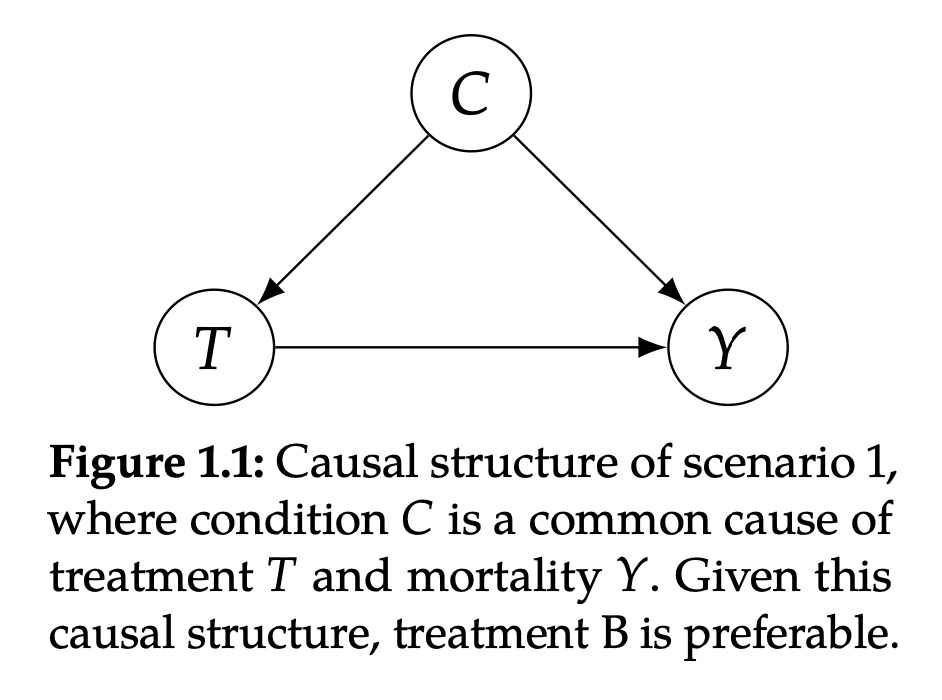
Figure 1.1

As shown in Figure 1.1, C (Condition) is the common reasons for T (Treatment) and y (outcom). Here C represents the severe condition. T represents the treatment plan. Y represents whether it dies. This Graph means that the severe severe condition will affect what kind of solution will the doctor use, and the severe condition itself will cause death. Treatment B is more effective in reducing mortality.

In this case, the doctor decided to provide a solution to most people with mild illness, and left more expensive and limited B the treatment methods to those with serious illness. Because people with severe condition are more likely to die (C → Y in Figure 1.1), and a person is more likely to receive B therapy (C → T in Figure 1.1). Therefore, the reason for the higher mortality rate of the overall B is only the majority (500/550) in the selection scheme B is the most ill, and even if the more expensive solution B is used, the mortality rate is 100/500 = 20% is lighter than lighter than lighter than lighter than lighter. The mortality rate of the symptoms B is 5/50 = 10% high, and the final mixing result will be more inclined to the result of severe illness. Here, Condition C confuses the effect of Treatment T on mortality O. In order to correct this mixed factor, we must study the relationship between T and Y of patients with the same conditions. This means that the best treatment method is to select low mortality treatment methods in each sub -group (Table 1.1) in Table 1.1: Plan B.

SCENARIO 2

Figure 1.2

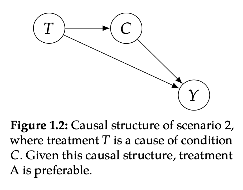
As shown in Figure 1.2, T (treatment scheme) is the reason for C (the severe disease), and C is the reason for Y (death or not). The actual scenario of this situation is: Plan B is very scarce, so that patients need to wait for a long time after choosing to receive treatment to be actually treated, and patients who choose A will soon be treated. In this case, the treatment plan has nothing to do with the condition, and the situation one, the condition will determine the plan.

Because the condition of COVID-27 patients will deteriorate over time, Plan B will actually cause patients with a lighter condition to develop into severe illness, which will lead to higher mortality. Therefore, even if B is used as more effective than A (Figure 1.2 in Figure 1.2 T), due to the long -term waiting of Plan B, it will cause the disease to deteriorate (negative effects in Figure 1.2 T → C → Y) 550 options for 550 options. There are 500 people in B. Because they have been waiting for a long time, only 50 are mild, so the results of Total's results will be more biased to B's severe mortality rate 20%. Similarly, the 16% mortality rate of Total A will be more biased towards A's mild mortality 15%.

At this time, the optimal choice is solution A, because Total's mortality rate is lower. The results of the actual table are also consistent, because B treatment is more expensive, so choosing scheme B with a probability of 0.27 and the probability of 0.73 selected A.

In short, more effective treatment depends on the cause and effect structure of the problem. In Sites 1 (Figure 1.1), B is more effective. One of the reasons in Scenario 2 (Figure 1.2), A is more effective. Without causal relationships, Simpson's paradox cannot be resolved. With causality, this is not a paradox.

1.2 Application of causal inference

Cause and effect inference is essential for science, because we often want to put forward causal requirements, not just correlation requirements. For example, if we want to choose in a disease treatment method, we hope to choose a treatment method that can get cure for most people without causing too many bad side effects. If we want a reinforcement algorithm to get the greatest return, we hope that the action it takes can make it the greatest return. If we study the influence of social media on mental health, we will try to understand what the main reason for the result of a certain psychological health is arranged according to the percentage of the results that can be attributed to each reason.

Cause and effect inference is essential for strict decisions. For example, suppose we are considering the implementation of several different policies to reduce greenhouse gas emissions, but due to budget restrictions, we must choose only one. If we want to maximize the role, we should conduct causal analysis to determine which policy will lead to maximum emission reduction. For another example, we are considering taking several intervention measures to reduce global poverty. We want to know which policies will minimize poverty.

Now that we have learned about the general examples of Simpson's paradox and some specific examples in science and decision -making, we will turn to the difference between causality and prediction.

1.3 Related 性 Cause and effect

Many people have heard the mantra of "correlation does not imply caus". First explain why this is the case.

Figure 1.3

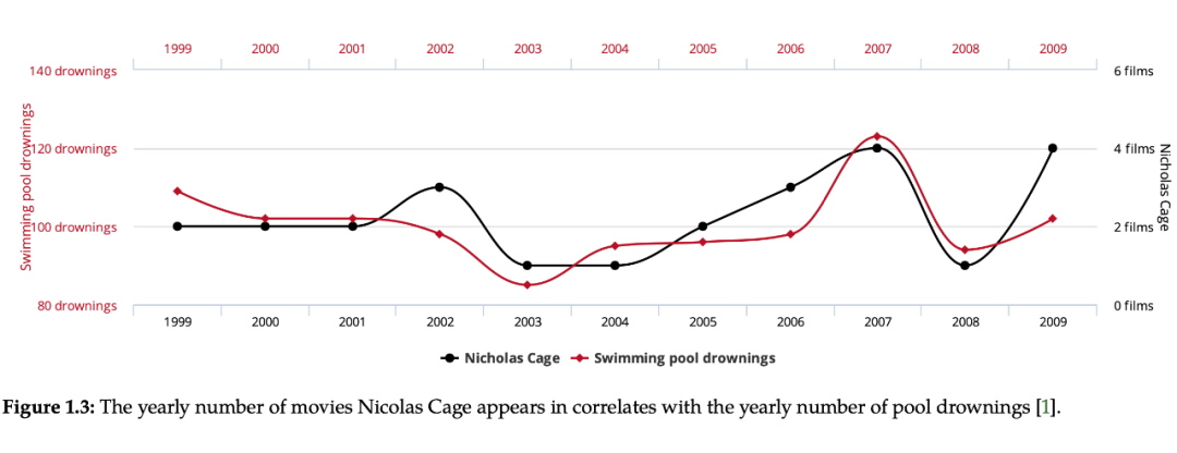
As shown in Figure 1.3, the number of drowns drowned for each year due to the swimming pool is highly correlated with the number of movies starring in Nicolas Cage each year. If you only look at this picture, you can get the following explanations: (1) Nicolas Cage encourages bad swimmers to jump into the swimming pool in his movie. (2) When Nicolas Cage saw how much drowning happened that year, he was more motivated to play more movies. (3) Maybe Nicholas Cage is interested in increasing his popularity among the cause and effect reasoning, so he returned to the past to convince him to make a correct number of movies in the past and let us see this correlation, but it is not fully matched. Because this can cause doubt, which prevents him from manipulating the correlation with data in this way. However, as long as a common sense person knows that the above explanations are wrong, there is no causal relationship between the two, so it is a false correlation. From this simple example, we can intuitively understand that "correlation is not equal to causality."

1.3.1 Why is correlations not equal to cause and effect

Note: "Correlation" is often used as synonymous with speaking as statistics. However, "association" is only a measure of Linear Statistics Dependency in theory. In the future, we will use the word Association to represent Statisticsical Dependency.

For any given number association, it is not "all associations are causal relationships" or "no association is causal relationship". There may be a large number of associations, and only part of them are causal relationships. "Related is not equal to causality." It means that the number of associations and the number of cause and effect can be different.

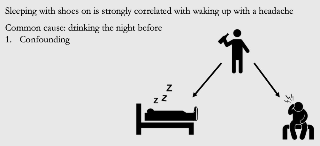
Consider another example. It was found that in most cases, if someone wore shoes to sleep, it would have a headache after waking up. In most cases, if you don't wear shoes to sleep, you don't have headaches after waking up. If you do not consider cause and effect, people explain such related data as "wearing shoes and sleeping can cause people to wake up headaches, especially when they are looking for a reason to prove that it is reasonable to not wear shoes to sleep.

Figure 1.4

In fact, they are all caused by a common reason: drinking the night before (drunk because of the probability of wearing shoes to sleep). As shown in Figure 1.4, this variable is called "Confounder" or "Lurking Variable". We will be called Confounding Association, which will be caused by Confounder, which is actually a false association.

The Total Association observed can be composed of a mixed -associated Confounding Association (red arrow in the figure) and causal association (blue arrow in the figure). The possible situation is that wearing shoes and sleeping really have a cause and effect of headache after waking up. Then, the total connection will be not just mixed, nor is it just cause and effect. It will be a mix of the two. For example, in Figure 1.4, causal relationship flows along the blue arrow that wakes up from wearing shoes to headache. The mixed association flows along the red path from wearing shoes to drinking to headache. We will make a clear explanation of these different types of associations in Chapter 3.

1.4 Some concepts involved

STATISTICAL VS. CAASAL sometimes cannot calculate some causal amounts even if there is unlimited data. In contrast, many statistics are about uncertainty in solving limited samples. When given unlimited data, there is no uncertainty. However, association is a statistical concept, not a causal relationship. Even if there is unlimited data, there are more jobs to do in terms of causal inference.

Identi i Cation (identification) vs. Estimation (estimated) identification causality is a unique content of causal reasoning. Even if we have unlimited data, this is a problem to be solved. However, causal push -ups also have common estimates with traditional statistics and machine learning. We will start with the recognition of causal relationships (chapters 2, 4, and 6), and then turn to the estimation of causality (Chapter 7).

Intervental (intervention) vs. Observational (observation) If we can intervene/experiment, the recognition of causal relationships is relatively easy. This is because we can actually take the actions we want to measure causality, and simply measure the causality after we adopt the operation. However, if only observation data is observed, it is difficult to identify causality because there will be the existence of the Confounder mentioned earlier.

2. Potential results POTENTIAL OUTCOME2.1 Potential result independent causal effect

First introduce these two concepts through two examples.

Scenario 1: Suppose you are unhappy now. And you are considering whether to raise a dog to become happier. If you become happy after raising your dog, does this mean that the dog makes you happy? And if you don't have dogs, you will also be happy? In this case, dogs are not a necessary condition for you to be happy, so it is not right to have a causal effect on you. SCENARIO 2: Another situation is that if you become happy after raising dogs. But if you don't get a dog, you will still be unhappy. In this case, dogs have a strong causal effect with you.

Use Y to represent the result-happiness, means happy, < /g> < /g> indicates unhappy; indicates that there are dogs, means no dog. < /g> < /g> indicates that if you have a dog, then you will observe your dog to raise a dog Later is the happiness index.

< /g> < /g> indicates that if you have no dog, then you will observe without a dogHappiness index.

In SCENARIO 1, < /> < /> g data-mml-node = "mn" transform = "translate (5471.2, 0)" /> < /g>; In SCENARIO 2, < /g> < /g>.

The < /> < />g data-mml-node = "mn" transform = "translate (3637.7, 0)" /> < /g> < /g>/g> is the Potential Outcom.

In terms of formalization, Potential Outcome < /g> refers to if you adopt Treatment < G Stroke = "CurrenTColor" Fill = "Currencolor" Stroke-Width = "0" Transform = "MATRIX (1 0 0-1 0)"> , what will your results be. POTENTIAL OUTCOME data-mml-node = "mi" /> < /g> < /g> and Observed Outcom The difference is that not all POTENTIAL OUTCOME have been observed, but may be observed. For separate individuals , Individual Treatment Effect (ITE) Independent causality effect is defined as:

As long as there are more than one individual in the population, < /g> is a random variable, Because different individuals will have different POTENTIAL OUUTCOME. In contrast, < /g> < /g> < /g> It is usually regarded as non-random variables because the bidding means that we restrict attention to a single individual (in a specific background), and its Potential Outcom is certain.

ITE is a major indicator we care about in causal inference. For example, in the above scenario 2, you will choose to raise dogs, because the cause and effect effect of dogs for your happiness are positive: < /> < /> g data-mml-node = "mo" transform = "translate (4915.4, 0)" /> . On the contrary, you may choose not raising dogs in Scenario 1, because the dog's happiness has no causal effect: "> . 2.2 Basic issues in causal inference

The basic problem in causal inference is that if the lack of data is obtained to obtain causal effects.

That is, we cannot observe at the same time < /g> < /g> < /g> < /g> and < /g> ,

Then we cannot get < /g> < /g> < /g> , the causal effect cannot be judged. This question is unique to causal inference, because in causal inference, we are concerned about how to propose Claim, and these Claims are defined by Potential Outcome.

No (not) Potential outcome observed is called Countfactuals because they are opposite to facts (reality). "POTENTIAL OUTCOME" is sometimes called "Countfactual Outcome". But this book will not be called like this. The author believes that a Potential Outcome < /> < /> g data-mml-node = "mi" transform = "translate (1152, 0)" /> < /g> /g> Observed another Potential Outcom It will not become anti -facts before. The observed POTENTIAL OUTCOME is sometimes called factual Factual. Please note that before the results were observed, there were only potential results, no anti -facts or facts. 2.3 How to solve basic problems 2.3.1 Average causal effect Lack of data explanation

Since the independent causal effect cannot be obtained, can the average causal effect be obtained (ATE)? In theory, you can get expectations:

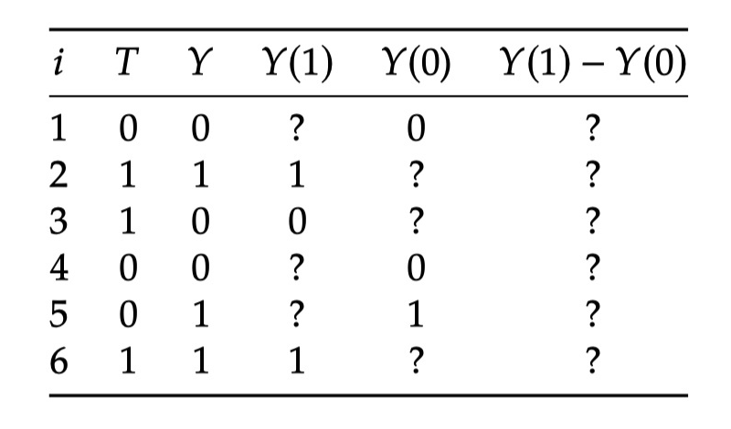
Table 2.1

But how do we actually calculate ATE? Let's take a look at some fabricated data in Table 2.1. We use this table as the entire population of interest. Due to the basic issues of causality, some missing data are caused. All in the table? They all said that we did not observe this result.

From this table, it is easy for us to calculate the associational di ff EricE (through the Type and Y column):

Through the expected linear computing law, ATE can be written:

At first glance, you may first get it directly

But in fact, this is a wrong approach. If this publicity is established, it means that "cause and effect is associated", and we have refuted in the first chapter.

Take the example of wearing shoes to sleep in the first chapter as an example.

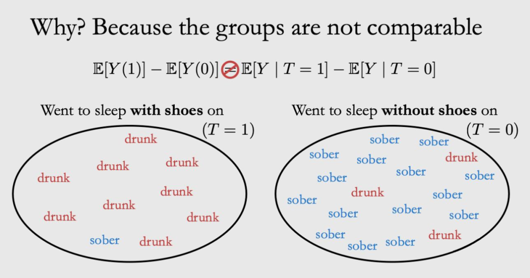
In T = 1, most of them drink alcohol, and most of T = 0 are not drinking. T = 1 and T = 2 Subgroup is uncomparable. E [y | t = 1] must be greater than e [y (1)], because drinking will be more likely to have a headache.

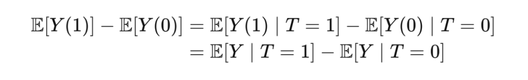
So what does the two groups of Comparable look like? As shown in the figure below, at this time, the two formulas can be equated.

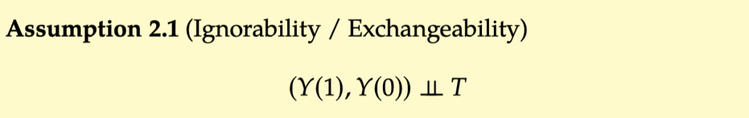
2.3.2 Ignorability Exchangeability

At this time, we can ask the most important question in this chapter, "What kind of assumptions can make ATE = AssociationAL ff EricE"?The same is equivalent to "What assumptions allow us to take < /g> < /g>(Ignoring the question mark) minus the < /g>) Come to calculate ATE? "

The answer to this question is to assume that < /> < /> g data-mml-node = "mo" transform = "translate (4804.4, 0)" /> < /g> < /g> /g>, that is, Potential Outcom < /g> < /g> and treatment independence. This assumption enables us to simplify ATE to associational di ff EricE, that is, with the following derivation:

The first = set up by < /> g data-mml-node = "mo" transform = "translate (4526.7, 0)" /> < /g> The second = set up because of < /g> , POTENTIONL OUTCOME < g data-mml-node = "mi" /> < /g> < /g> < /g> 2.13 Explanation. You can understand from two aspects that the independence of 2.1: Ignorability and Exchangeability.

IGNORABILITY:

This neglect of missing data is called ignored iGnorability. In other words, iGnorability is like ignoring how people ultimately choose the Treatment they choose, but just assume that they are randomly assigned Treatment, that is, the effect of removing the Confounder, that is, g data-mml-node = "mo" transform = "translate (763, 0)" /> < /g>; "Currentcolor" file = "Currentcolor" stroke-width = "0" transform = "matrix (1 0 0-1 0)"> < /g>. Fig 2.1

Fig 2.2

Exchangeability:

Another angle about this assumption is exchanging Exchangeability. Exchangeability means that the individual in the Treatment Group is exchanged, that is, if they are replaced, the new experimental team will observe the same results as the old experimental group, and the new control team will observe with the same as The old control group is the same. Formally, exchanges mean:

Then you can launch:

This and < /> < /> g data-mml-node = "mn" transform = "translate (3637.7, 0)" /> < /g> equivalent. An important intuition about exchanging is that it guarantees the comparable of the experimental group. In other words, the experimental team is the same as all aspects other than Treatment. This intuition is the basis of the concept of "control" or "adjustment" variables. We will soon discuss this issue when discussing conditions. Understand Exchangeability with visual examples:

All individuals of T = 1 are called Group A, and all individuals of T = 0 are called Group B. After exchanging the individuals in groupa and groupb, Observe Outcome remains unchanged.

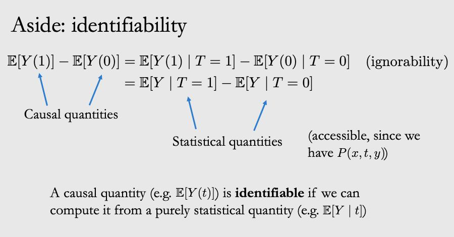
Then the < /g > Keep unchanged, and then you can launch independence. Let's introduce a concept: Identifiability

If an expression of a causal effect can be reduced to a pure statistical expression, only statistical symbols, such as T, X, Y, expectations, and conditions to represent = "Currentcolor" Stroke-Width = "0" Transform = "Matrix (1 0 0-1 0)"> < /g> of.

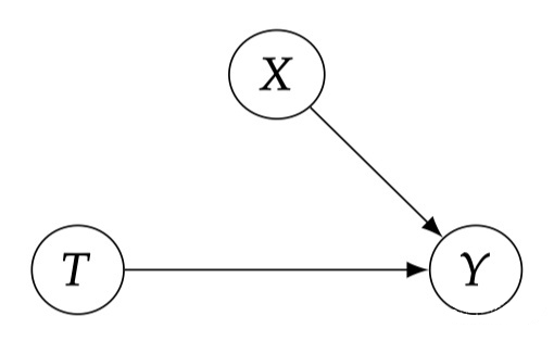
We have seen that 2.1 has a very good nature. However, in general, it is completely unrealistic, because there may be mixed factors in most data we observe (Figure 2.1). However, we can implement this assumption by conducting random experiments RCT. Random experiments forced Treatment not to be caused by any other factors, but determined by coins, so we have the causal structure shown in Figure 2.2. We discuss random experiments more deeply in Chapter 5.

From two angles, this section introduces assumptions 2.1: neglect and exchangeability. Mathematically, these two assumptions mean the same, but their names correspond to different ways of thinking about the same hypothesis. Exchangeability and negligence are just the two names of this assumption. After that, we will introduce this hypothesis more practical and conditional version.

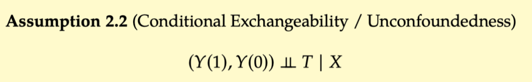
2.3.3 Conditional Exchangeability Unconfoundededness

The above example is explained. 2.2 is: "Among all drunk people, it is not determined by its subjective consciousness, but has nothing to do with consciousness. It is determined by a hidden hand of God." There are two different explanations for the same way.

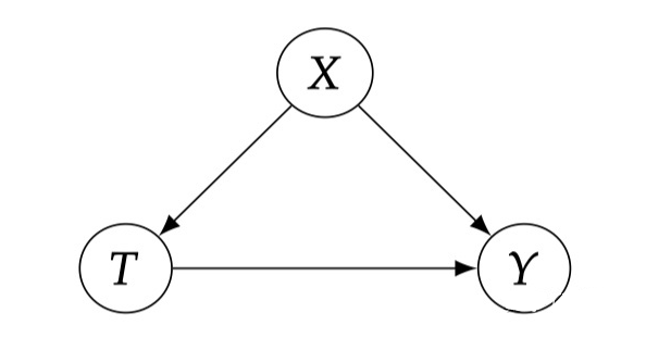
Conditional Exchangeability: In observing data, it is unrealistic to assume that the experimental group can be Exchangeability. In other words, there is no reason to expect that each group is the same on all related variables other than Treatment. However, if we control the relevant variables through conditionalization, the experimental group may be exchanged. In this case, although Treatment and Potential Outcome may be unconityally associated (because the Confounder exists, red dotted lines), they are not associated under the condition of X fixed (imagined that the red line is cut off).

As shown in FIG 2.3, X is the confunder of T and Y. Therefore, there is a one between T and Y. 0 0-1 0) "> < /g> < /g>. However, when we are continginging on x, that is, the value of X is fixed, and the Non-Causal Association between T and Y will be dropped by the block and turned into:

We can launch CAUSAL Effect under the X fixed conditions, that is, the Conditional Average Treatment Effect:

The first line is the expected formula, the second line is obtained by hypothetical 2.2, and the third line is obtained by observation data.

At this time, if you look forward to X, you can get a complete Average Treatment Effect. This is also called Adjustment Formula (adjustment formula):

Conditional Exchangeability (Assuming 2.2) is the core hypothesis of causality, and it has many names. For example, unconfoundedness has no mixing, Conditional Ignorability conditions, no unobserved confounding, and Selection on Observables. We will use the name "unconfoundedness no mix" in this series of tutorials.

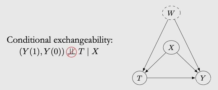
However, the actual situation is that we usually cannot determine whether the conditions for the conditions are established. There may be some unspeakable mixed factor that is not part of X, which means that the conditions that violate the conditions can be exchanged. As shown in the figure below, because there is another mixed factor W, the independence does not exist.

Fortunately, random tests can solve this problem (Chapter 5). Unfortunately, this situation is likely to exist in observation data. The best thing we can do is to observe and fit the collaborative variables (x and w) as much as possible -to ensure the Unconfoundedess as much as possible.

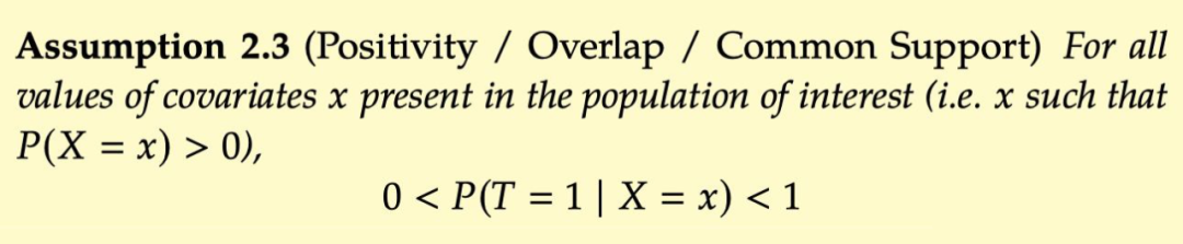
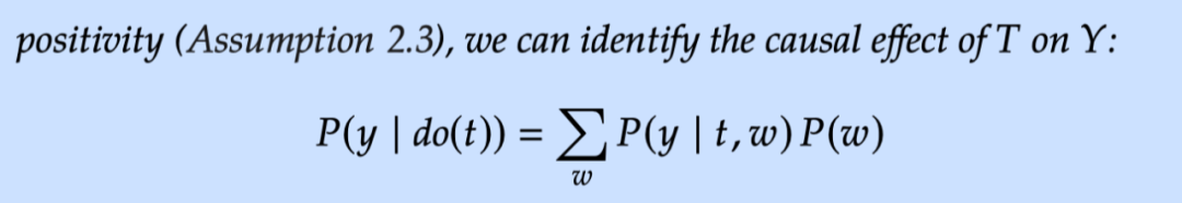
2.3.4 Positivity/Overlap and Extraporation, which is imagined to perform the unconfoundededness, but it may actually have side effects. This is related to another assumption that we have not yet discussed: Positivity enthusiasm. POSITIVITY means that any group with different collaborative value x = x has a certain probability of accepting any value Treatment. That is, . In order to understand the original text, it is recommended that you stop and look back carefully. Positivity is the condition that all subgroups of the data with different covariates have some probability of receiving any value of treatment. Formally, we define positivity for binary treatment as follows

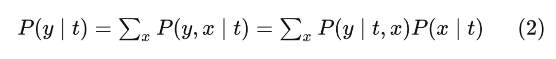
The following explains why Positivity is important, first review the adjustment formula:

If you violate the posity, then or < /g> < /g>,

Obtain or "> , which corresponds to two events in the adjustment formula. Change the expectations in EQ. (1) to sum up, EQ (1) can be written as:

Apply Bayes Rule, you can get:

In EQ. (2), if the , then it won't be a causal effect. The intuitive explanation is that if , then it means that in the group group of x = x, everyone accepts Treatment (each drunk every drunk People wore shoes to sleep), so that causal effect cannot be calculated.

The Positivity-Unconfoundedess Tradeo ff:

Although more coordinated variables may have a higher chance of satisfying Unconfoundedness, there will also be a greater chance of violating Positivity.As we increase the number of collaborative variables, each subgroup is getting smaller and smaller, and the possibility of the entire subgroup is getting the same time.For example, once the size of Subgroup is reduced to 1, it will definitely not satisfy Positivity.2.3.5 no interference, consistency, and suba

A few other concepts are introduced in this section:

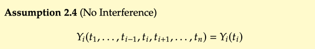
No interference:

No Internet refers to the Potential Outcom of each individual only related to the Treatment received by the current individual, and has nothing to do with the Treatment of other individuals.

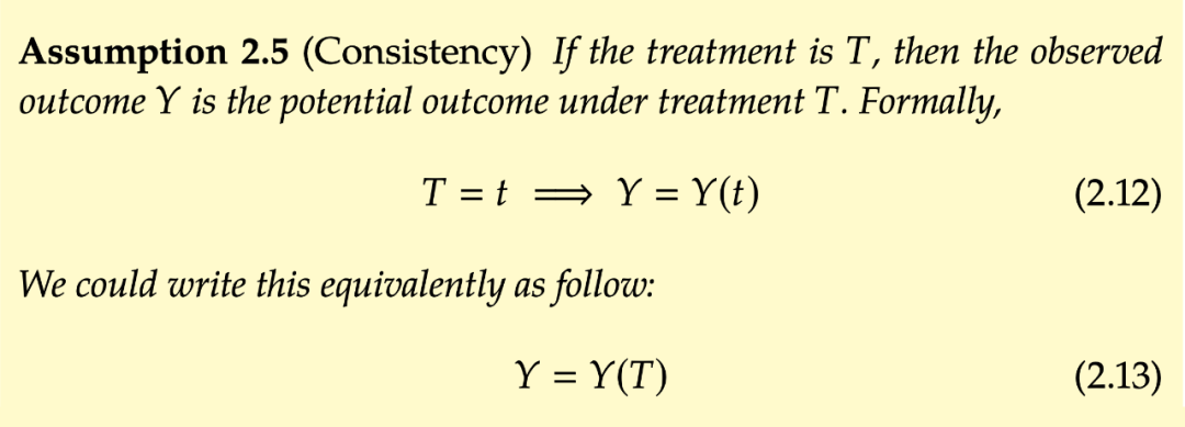
Consistency:

Consistency consistency refers to the time of the observed time T = T, the result of observation y is actually the Potential Outcom-y (t) of T = T. In this way, you can explain why < /g> "> < /g> < /g>, which may solve some of the previous parts The question left by the reader is why 2.3.6 TYING It All Together

After understanding the above assumptions, let's review the adjustment formula again.

This is how to combine all these assumptions to ensure the recognition of the average causal effect ATE. Through the above formula, it is easy to count the actual valuation of ATE.

3. What is a picture in the causality and association flow in the figure?

I guess my friends who have seen this series of articles are already familiar with the concept of Graph, and I won't talk about it here. The figure is a data structure composed of node node and edge Edge. Let ’s put a few examples of ordinary types: below:

3.2 Bayesian Network

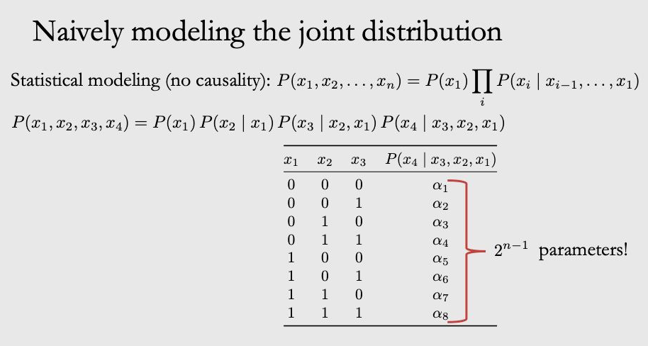
Many of the tasks of causality models are done on the basis of probability graph model. To understand the causal diagram, we must first understand what the probability graph model is, although there is a big difference between the two. Bayesian network is the most important probability graphic model. Causal models (causal Beats Networks) inherit most of their attributes. The combined probability distribution can be written in the following form through the chain rule:

If you model the above formula directly, the number of parameters will explode.

If Only dependence on < g data-mml-node = "math">

That is, < /g> < /g> < /g> < /g> You can write < /g> < /> < /> g data-mml-node = "msub" transform = "translate (2949.1, 0)"> . We can use Graph to represent the dependent relationship between variables, this Graph is called Bayesian network. Generally speaking,

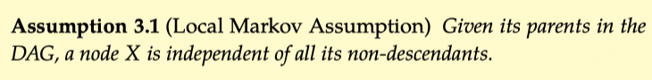
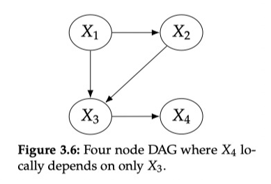
The nodes of the Bayesian network are random variables in the nodes in the ringless graph DAG. They can be observed variables, or hidden variables, unknown parameters, etc. Given DAG, how to calculate the combined probability distribution of all variables? The following assumptions need to be used, that is, the X node is only related to its parent node, and it has nothing to do with other nodes:

In this way, the combined probability distribution of Figure 3.6 can be written as the following form:

3.3 Causal map

The previous section was about statistical models and associated modeling. In this section, we will use causal leaves to enhance these models and turn them into causal models, enabling us to study causal relationships. In order to introduce causal fakes, we must first understand "What is CAUSE".

According to the above definition, if the variable y can change with the change of X, it is called the reason for x. Then give the entire book (strict) causal hypothesis 3.3. In the direction, each node is the direct reason for its sub -node. X is the parent node of Y, x is the direct reason of Y, and the reason for X (the parent node of X) is also Y, but it is indirect reason.

If we take all the direct reasons of Y, then any other reasons to change Y will not cause any changes in Y. Because the definition of CAUSE (De fi NITION 3.2) means that CAUSE is related to its E -ECT, and because we assume that all parent nodes are their sub -nodes, the parent nodes and sub -nodes in the causal map are related.

Non -strict causal relationship assumptions that some parent nodes are not the cause of their sub -nodes, but it is not common. Unless otherwise explained, in this book, we will use the "causal map" to refer to the DAG that meets the hypothetical assumptions of strict causality and omit the word "strict".

To sum up, DAG has a special form of Graph without a loop. Bayes network and causality are represented by DAG, but the meaning of the two is different. Dependent relationships, and causal diagrams express the causal relationship between variables. Because the edge of the cause and effect also implies a correlation between the two variables, so there is both causality and relationship in DAG, which also corresponds to the topic of this chapter.

3.4 The simplest structure

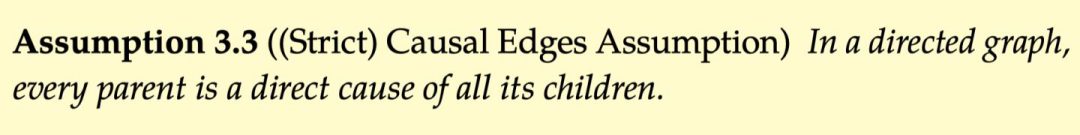
Now we have already understood the basic assumptions and definitions, and we can enter the core of this chapter: association and causality in DAG. First I start with the basic structure of DAG. These smallest constructs include the Chain chain (Figure 3.9A), FORK fork (Figure 3.9B), IMMORALITIES collision (Figure 3.9C), two unconnected nodes (Figure 3.10), and two connected nodes (Figure 3.1111 To. Its schematic diagrams are shown below

In a Graph (Figure 3.10) consisting of two unlimited nodes (Figure 3.10), and It must be independent independent, unreasonable Unassocity.

Instead, if there are edges between the two nodes (Figure 3.11), then it must be associated. The assumption 3.3 is used here: Because X1 is X2, X2 must be able to respond to the change of X1, so X2 and X1 are associated. Generally speaking, if the two nodes are adjacent in the causal map, they are all related.

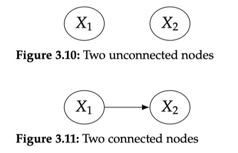
3.5 chain fork structure

Putting the chain chain and fork for the introduction in a section because the characteristics of both are the same.

Correlation:

In Chain, X1 is the reason for X2, X2 is the reason for X3, then X1 and X2 are related. X2, X3 are related, and X1 and X3 are also related. In FORK, X2 is the common cause of X1 and X3, and X1 and X3 are also related. This may be a bit anti -intuitive. X1, X3 obviously have no edges. Why is there any connection? For example: increased temperature will lead to rising sales of ice cream, and at the same time, it will also increase the crime rate. From the perspective of the data of ice cream sales and crime rate, they have the same trend, so it is related, although there is no causality between them, there is no causality between them. relation.

Associated Flow is symmetrical, X1 and X3 are related, and X3 is also related to X1, that is, the red dotted line in the figure. The cause of causality is non -symmetrical, and it can only flow along the side, that is, X1 is the reason for X3, X3 is not the reason for X1.

Independence:

Chain and fork also have the same independence. If we fix X2, that is, Condition On X2, then the correlation between X1 and X3 will be blocked by blocks and become independent.

In Chain, if X2 is fixed to a fixed value, X1 does any change, and it will not affect the change of X2. Because it has been fixed, then the X3 will not change. Therefore, X1 and X3 become independent.

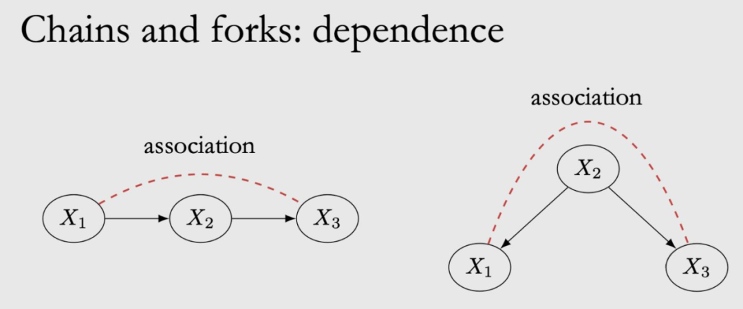
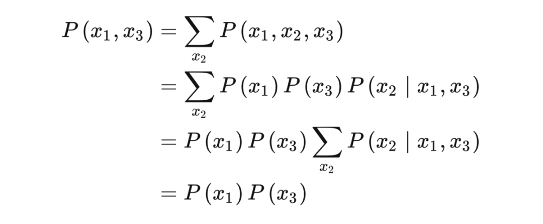
Proof:

The combination probability of China is distributed as follows:

Then, Condition On X2, use Bayes Rule to get:

再次利用 Bayes rule，得到：

From this conclusion, .

3.6 collision structure

The collision structure refers to the reason for X1 and X3 to be X2. X2 is also called Collider. In this case, X1 and X3 affect X2, but the information does not flow from X2 to X1 or X3, so X1 and X3 are independent of each other. < /> /g> < /g> The Association Flow was dropped by X2 Block, The red line in the figure is only half. Proof:

If X2 is fixed, that is, Condition On X2, at this time X1, X3 changed from independence. For inappropriate examples, X1 is wealth, X2 is a look, X3 is chasing girls, and handsome can be chased to girls. If someone does not chase the girl and we observe his handsome, then he must have no money. If he has money, he must not grow.

If the offer nodes, X1, X3 are also related to the ConDition On Collider nodes. You can imagine the X2's offspring nodes as an agent node of X2. Condition on proxy nodes are the same as Condition On X2.

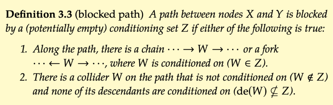
3.7 D-separation

First of all, the concept of Blockd Path is introduced to given the condition set.

This path exists in chain ( ) or exist ( ), and Condition On W width = "0" transform = "matrix (1 0 0-1 0 0)"> )

This path exists in a color w ( ), and all the offspring nodes of W's offspring are not fixed ( < /g>) Similarly, the definition of Unblock Path and Block Path on the contrary. There is no ASSOCIATION FLOW from X to Y in Block Path, which is dropped by Block. There is an association flow from X to Y in the Unblock Path.

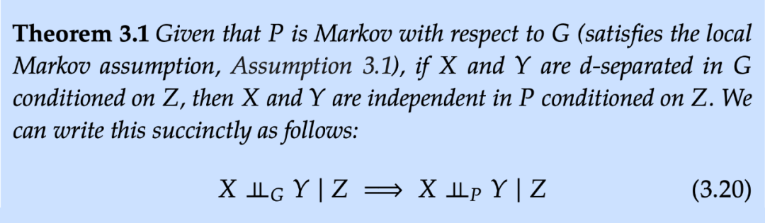
The concept of D-separation is given below:

Under the condition of a given set z, if the path between any two nodes in x and y is block, then X and Y are separated by Z d-separated. zhiyao exists in a UNBLOCK, then X and Y are connected by Z d-. If X and Y are separated by Z d-, you can get X and Y independent when giving Z. < /g> < /> < /> g data-mml-node = "mo" transform = "translate (3832.1, 0)" /> < /g> < /g> /g> Represents D separation, < /g> Independence. Small practice:

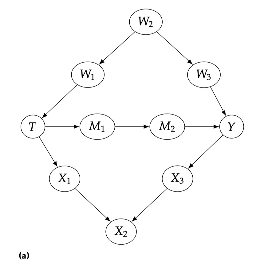
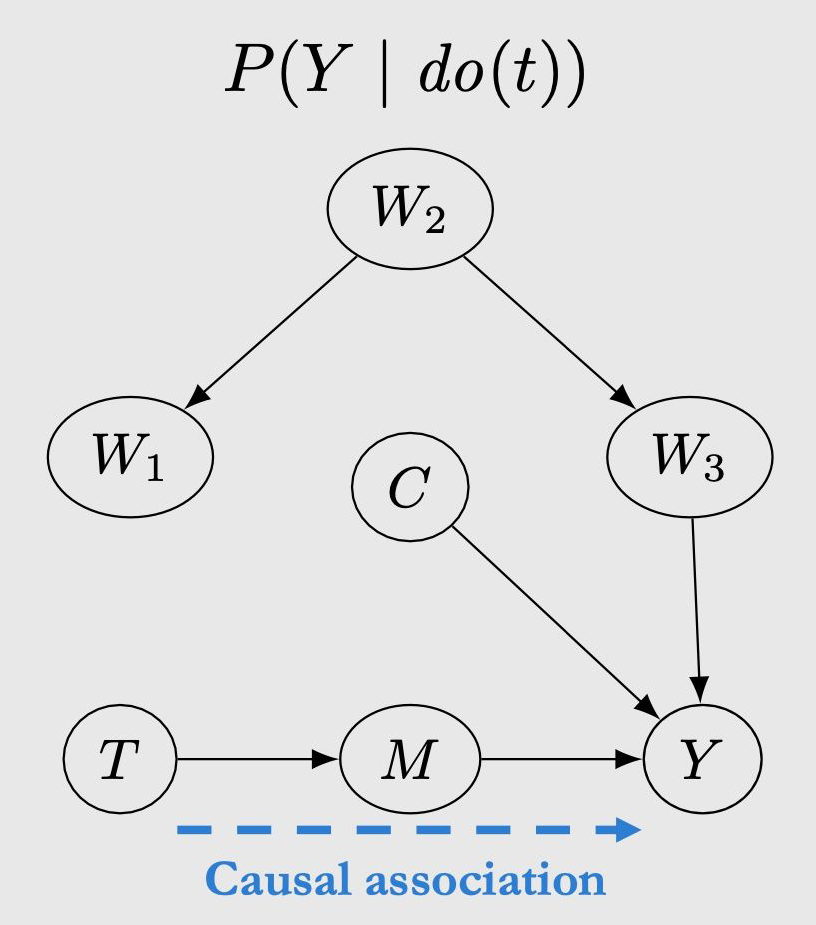
Determine whether the following situation is D-separation

1. Are T and Y D-seaParated by the Empty Set?

NO

2. Are T and Y D-seaParated by W2?

NO

3. Are t and y d-separated by w2, m1?

Yes

4. Are t and y d-separated by w1, m2?

Yes

5. Are T and y d-separated by w1, m2, x2?

NO

3.8 Cause and effect flow and association flow

Finally, summarize the causal flow and associations on the figure below. Related flow flows along the Unblock Path, and the causality flows along the side. We will call the causal association as causal association. The overall Association includes Causal Association and Non-Causal Association. An example of a typical non -causal correlation is Confounding Association.

Common Bayesian networks are pure statistics models, so we only talk about the flow flow on the Bayesian network. However, the flowing method associated in the Bayesian network is exactly the same as the flow method in the causal map. The association is flowing along the chain and the fork, unless the CONDITION ON mid -node, and the Collider will prevent the flow of the association, unless it is concessively On colorider. We can determine whether they are associated with two nodes by D-separation (the relationship between the two). The special thing about causality is that we also assume that the side has causal significance (causal assumption, assumption 3.3). This assumption will introduce causality into our model. It makes a type of path a new significance: there is a path. This assumption gives a unique role in the path, that is, the causal relationship along them. In addition, this assumption is asymmetric; "X is the reason for Y" and "Y is the reason for X" is different. This means that there is an important difference between association and cause and effect: association is symmetrical, and causality is asymmetric.

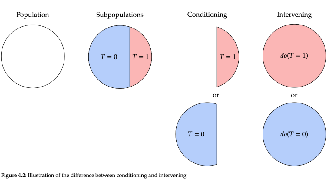
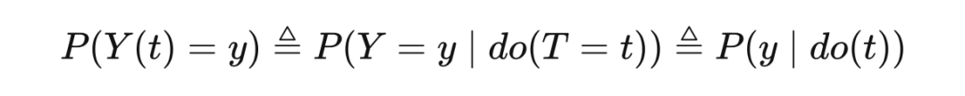
4. Cause and effect models, do operator, intervention 4.1 DO operator and intervention in probability, we have ... Condition on, but this is different from intervention. With The condition only means that we will pay attention to the part of the crowd that restrictions on the overall population to accept Treatment = T. In contrast, intervention intervention allows the overall population to accept Treatment = T, regardless of whether the time of the observed itself is T. Usually use the Do operator to represent intervention operations, that is, the overall population accepts Treatment = T equivalent at g data-mml-node = "mo" transform = "translate (2375.8, 0)" /> . You can deepen the understanding compared with Figure 4.2. Subpopulations indicates that the blue part observed in the data observed is the collection of T = 0, and the red part is the collection of T = 1. CONDITIONG said we only pay attention to the blue parts or red parts. Do (t = 1) refer to the blue part of T = 0 into T = 0, that is, red.

Remember the potential results of Potential Outcome, which is mentioned in Chapter 2, < /g> < /g> It is equivalent. < /g> The distribution can be written: the average causal effect ATE can be written in the following form to be written in the following form. The

We are more concerned about < g data-mml-node = "mi" /> "> Instead of its average value, with the probability distribution, the expectation will naturally find out. We will < /> < /> g data-mml-node = "mi" transform = "translate (5080.1, 0)" /> and other probability distribution containing Do operators is collectively referred to as intervention distribution interventional distributions.

Intervention distribution < /> < /> g data-mml-node = "mi" transform = "translate (5080.1, 0)" /> 和观察分布observational distribution There are essential differences.

Observation distribution < /g> < /g> or There is no do operator, so we can directly obtain from the observed data without having to do any additional experiments. If the expression containing the DO operator can be simplified, the Q is not included in the form of DO, then Q is recognized by identifying IDENTI fi ABLE.

Whenever, whenever the do operator appears in "｜", everything in the expression is obtained after intervention measures (that is, post-intervention). For example, < /g> "> < /g> It means < /g> In SubSet, the time of all individuals is equal to the expectations of y after T.

Instead, < /g> indicates that in The expectations before I.E. Pre-intervention in this subset. The difference between the two is very important for the anti -facts to be introduced in the future.

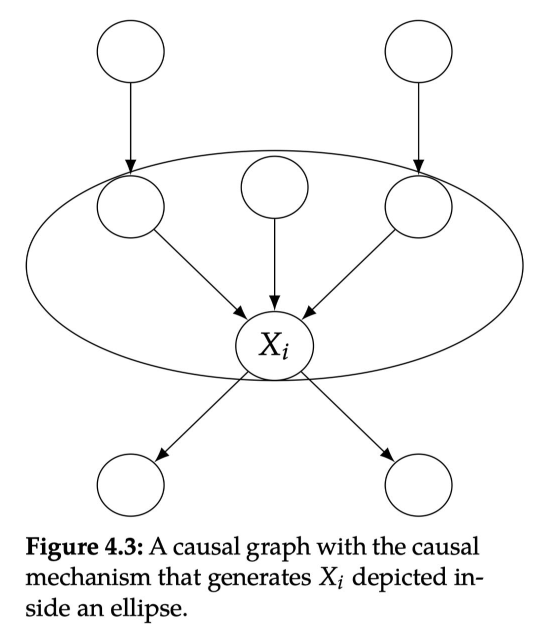
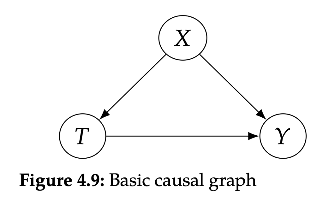
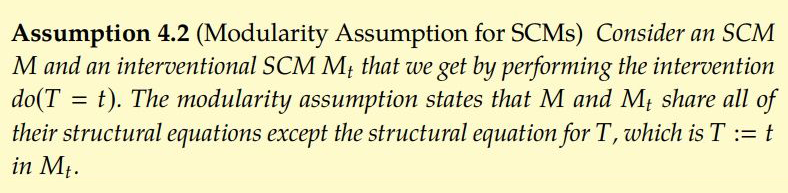
4.2 Modularity Module hypothesis Before introducing this very important assumption, we must specify what the causal mechanism is. There are several different ways to consider causal mechanisms. In this section, we will produce The causal mechanism is specified as The conditional probability distribution < /g> .

As shown in Figure 4.3, The causal mechanism is all Parent node and its pointing to The side. The modular assumption refers to: assuming that the variable Intervention will only change is limited to the ellipse in the figure and will not change it. Generate any causal mechanism for any other variables. In this sense, the cause and effect mechanism is modular. The clear definition of the modular assumption is as follows:

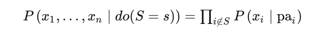
If the node collection S intervention, set the variables as a constant, for any node I:

If the node I is not in the collection S, then the conditional probability distribution remains unchanged

If the node I is in the collection S, if is the variable The value specified after being intervened, then < /g> Essence

The second point can also be said that if Inform with intervention ( is consistent with the intervention ( < g data-mml-node = "mi"/> equal to < g data-mml-node = "msub">

Then < /g> < /g> < /g> Modification assumption allows us to only be in one picture in one picture You can enter different intervention distribution. E.g

These three completely different distributions can be distributed < g data-mml-node = "math"> < /> < /> G> shows that except for the factor involved in intervention, other factors are the same.

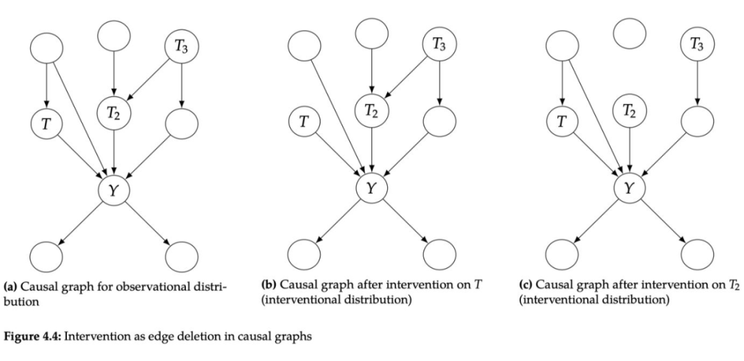
The causal diagram of the intervention distribution is the same as the combined distribution, but it is just removed all the edges pointing to the intervention node: this is because the conditional probability distribution of the intervention node < /g> < /g> < /> < g data-mml-node = "mi" transform = "translate (4739.5, 0)" /> < /g> is already 1, so we can ignore the factor. Another explanation is that since the intervention node has been set to a constant, it will inevitably be affected by the parent node, so the causal relationship between the between it can be removed. The diagram of the deleted edge is called ManipularEd Graph. Taking Figure 4.4 as an example, the corresponding (b) of T intervention (b), to < g data-mml-node = "math"> intervention corresponds

Looking back at the decomposition form of the combined probability distribution in the Bayesian network:

Now intervention in node collection S, for < /g> , < /> < /> g data-mml-node = "msub" transform = "translate (1140, 0)"> < /g> < /g> The value before intervention is the same.

For < /g> , < /g> < /g> Therefore, the probability distribution after intervention can be expressed as (truncated factor decomposition): 4.3.1 example

Taking the simplest causal diagram of Confounder as an example, the combined probability distribution can be expressed as:

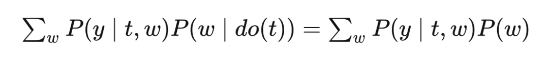
After intervention on T, < /g> < /g>, then the edge probability distribution of y is:

By comparative intervention distribution and normal conditional probability distribution, it can be more deeply understood why "association is not cause and effect"

It can be seen that the difference between EQ (2) and EQ (1) is that one is < /g> The other is < /g> < /g>. This example is more simplified. Suppose T is a two -value variable, we want to calculate ATE.

Because is PotentialoutCome < /g> < /g> The probability distribution, so you can get ,

Similarly, you get , the average effect effect ATE can be written as: if EQ (1) is substituted, the ATE can be completely written in the form of probability. The expression does not include DO, which can be obtained by observing the data. In this way, ATE can be obtained. In this way, ATE can be obtained.Is IDIFIED.We will describe this process more formally in the next section.

4.4 Back door adjustment 4.4.1 Back door path

The above figure is an example. Looking back at the third chapter, there are two association from T to Y, one of which is The other is the g data-mml-node = "mo" transform = "translate (981.8, 0)" /> < /g> < /g> < /g> < /g> < /g> and < /g> < /g> The non -causal association of G>, also known as the two paths is Unblocked (because it is a fork structure,

And there is no consition on). The meaning of the back door path is that if a path from T to Y is unblocked, and there is a edge of T (that is, < /g>), then this path is the back door path. Why is it called the back door? Because this path does not have an direction from T to Y, but because there is a edge pointing to T, it is equivalent to entering the back door of T. This path is opened. At this time, if we intervene in T, any edge point to T will be removed, the back door path will be blocked, and only cause and effect between T and Y will be associated.

If Condition On W1, W2, W3, and C, the back door path is also blocked.

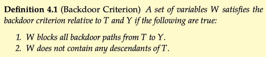
4.4.2 Back door criterion, if we want to bring < /g> < /g> The form of a full probability requires the W to meet the back door criteria.

For T and Y, if the following conditions are True, the variable collection W meets the rear door criteria:

Condition On W can block all the back door path between T and Y

W does not include all descendants of T

Introduce W to

Why , you can think about it like this.

The corresponding figure, because of intervention on T, all the edges pointing to T were deleted. Therefore It is only between T and Y only along the < /g> To.

In The corresponding figure, because of the Condition On W, all the back door paths are not blocked, T and Y There is only a connection along the path. In these two cases, the association flow only flows along there is a path, so it corresponds to the same conditional probability distribution. Because there is no point to T, T cannot affect W, so , so the upper formula can continue to be written:

This is the formula of the back door adjustment.

4.4.3 Relation to Potential Outcomes

Remember the adjustment formula introduced in Chapter 2:

Since they are all called adjustment formulas, is there any connection with EQ (3) in the back door? As for the expectations after the intervention:

Integrate T = 1 and T = 0:

You can see that EQ (4) and EQ (3) are equal. < /g> < /g> is the portal outcom < /g> < /g> Another representation. Of course, the establishment of EQ (3) also has a premise that Conditional Exchangeability: 4.5 Structure Cause and Effect Model

In this section, we will shifted from causal map models to structural causal models. Compared with a more intuitive diagram model, the structural causality model can explain more and clearly what is intervention and causality mechanism.

4.5.1 Structure and other Judea Pearls said that "=" in mathematics does not include any causal information, < /g> < /g> and < /g> < /g> It means the same meaning, "=" is symmetrical. But in order to express cause and effect, there is a needy symbol. If A is the reason for B, then changing A will definitely change B, but the otherwise is not established. We can use the structure of Structural Equation to indicate: here "=" is replaced with "=": = ". However, the mapping between B and A is certain. Ideally, we hope that it is probably probably, leaving room for some unknown factors. So it can be written as the following:

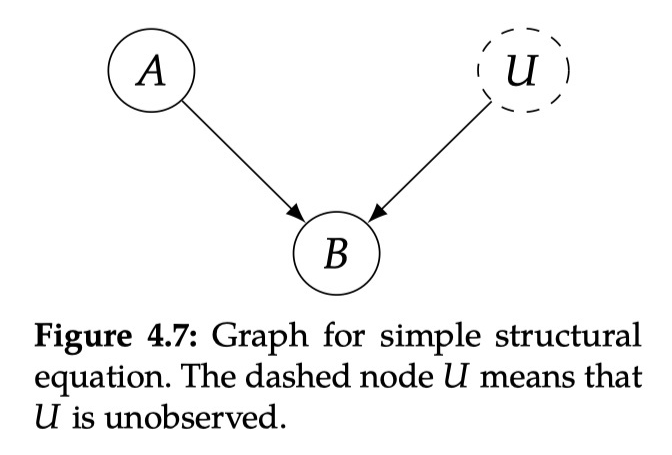
Among them, U is a random variable observed. In the figure, the dotted line is expressed in the figure that the u not observed is similar to the randomness we see through the sample individual; it indicates that all the relevant (noisy) background conditions of B are determined. The Function form of F does not need to be specified. When it is not specified, we are in a non -parameter state because we do not make any assumptions on the parameter form. Although mapping is certainty, because it uses random variable U ("noise" or "background conditions" variables) as input, it can represent any random mapping, so the structural equation is < /g> > promotion form. Therefore, when we introduce structural equations, cut off decomposition and backdoor adjustment are still established.

With the structure and other formulas, we can define the cause and causal mechanism more in detail. The causal mechanism for generating variables is the structural equation corresponding to the variable. For example, the causal mechanism for generating B is EQ (5). Similarly, if X appears on the right of the structure equivalence, X is the direct cause of Y. Figure 4.8 The more complicated structure and other formulas are as follows:

In the causal diagram, noise variables are usually hidden (dotted lines), not clearly drawn. The known variables when we write the structural equation are called endogenous variables, which are variables we are modeling causality -have parents' variables in causality. Instead, the exogenous variables are variables of no parents in the causal map. These variables are outside our causal model because we have not modeling and causality. For example, in the causal model described in FIG. 4.8, the endogenous variable is g data-mml-node = "math"> . The exogenous variable is < /g> < /> < g data-mml-node = "msub" transform = "translate (3409, 0)"> < /g> .

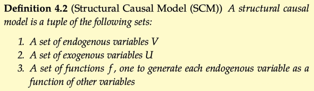
Structural causality model SCM is defined as follows, including a set of endogenous variables, a set of exogenous variables, and a set of functions that generate endogenous variables:

4.5.2 Intervention describes intervention from the perspective of SCM. Intervention in T Equivalent to replace the structure of T to . For example, the SCM corresponding to Figure 4.9 is: if you intervene in T to make it equal to T, then the SCM after intervention is:

It can be found that except for the structure of T itself, other equal forms remain unchanged. This is also determined by the modular assumption.

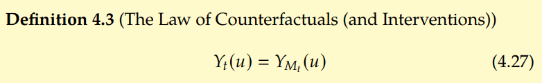
In other words, intervention operations are Localized. Through modular assumptions, Pearl can lead the guidelines for anti -affairs. Looking back at the concept of the potential result of the second chapter, < /g> < /g> refers to the individual I when Treatment = t Potential results. Here we change another mark to say that < /g> < /g>, where U is equivalent to i. According to the definition 4.3, the criterion of the anti -factual refers to the potential results and intervention of the treatment = t before intervention. 0) "> g data-mml-node = "mo" transform = "translate (2375.8, 0)" /> The potential results are equal. references

[1] Brady Next, INTRODUCTION to CAUSAL Inference from a Machine Learning Perspective, 2020

Edit: Yu Tengkai

- END -