Original | Google JAX help scientific computing

Author:Data School Thu Time:2022.09.17

Author: Wang Khan

Council: Chen Zhiyan

This article is about 3500 words, it is recommended to read for 9 minutes

This article introduces you to use Google JAX to help scientific calculations.

Google's latest JAX is officially defined as Numpy on CPU, GPU and TPU. It has an excellent Differentiation function and is a Python library that can be used for high -performance machine learning research. Numpy is very popular in the field of scientific computing, but in the field of deep learning, because it does not support automatic micro -score and GPU acceleration, it is more useful to use deep learning frameworks such as TensorFlow or PyTorch. However, the TensorFlow API launched by Google has some confusing situations. In the iteration of 1.X, there are different levels of APIs such as atom OP and Layers. In the face of different types of users, it is not a problem to use a multi -layer API with different particle size. However, the same level of APIs also have a variety of competitive products, such as Slim and Layers, they have improved learning costs and migration costs. JAX uses XLA to compile and run Numpy on accelerators such as GPU and TPU. It is very similar to the NUMPY API. Numby can do almost all things that can be done with jax.numpy, thereby avoiding the direct definition of the API.

The following briefly introduce several characteristics of JAX, and at the same time give some examples for readers to get started quickly. In the end, we will combine the scientific computing examples to show Google Jax's great power in scientific computing.

1.jax characteristics

1) Automatic differential score:

In the field of deep learning, the optimization of network parameters is achieved by gradient -based reverse communication algorithms. Therefore, it is very important to be able to achieve a differential point of any numerical function. The following examples are briefly introduced in conjunction with the official documentation.

First introduce the simplest GRAD for the first -order micro -score: you can directly find the gradient value of a function in a certain position through the Grad function

Import jax.numpy as jnp From Jax Import Grad, JIT, VMAP GRAD_TANH = Grad (jnp.tanh) [OUT]: 0.070650816

Of course, if you want to continue to find the second and third -order guidance for the dual -cut tongs, you can also do this:

Print (Grad (Grad (JNP.TANH)) (2.0)) Print (Grad (Grad (Grad (JNP.tanh))) (2.0)) [OUT]:-0.13621868 0.25265405

In addition, you can also use Hessian, JACFWD, and JACREV to implement functional conversion. Their functions are to solve the Haysen matrix and use forward or reverse mode to solve the Jacques matrix. Jacfwd and Jacrev can get the same result, but the efficiency is different in different situations, because this is because the corresponding micro -divided geometry behind the two and the pull back method. The GRAD mentioned earlier is based on the reverse mode.

In some optimization algorithms to be Newtonian, the second -order Hyen matrix is often used. To achieve the solution of the Haysen matrix. To achieve this goal, we can use JACFWD (JACREV (F)) or Jacrev (JACFWD (F)). However, the former is more efficient, because the inner Jacques computing is more appropriate to use the reverse mode by the derivative of the N -dimensional vector that is similar to a 1 -dimensional loss function. The outer layer is usually the guidance of the N -dimensional vector, and the positive mode is more advantageous.

2) Ob directionization

Whether in the study of scientific computing or machine learning, we will apply the defined optimization target function to a large amount of data, such as in the neural network to calculate the loss function value of each batch. JAX transforms automatically vectorization through VMAP, simplifying this form of programming.

The following combines several examples to explain this usage:

VMAP has 3 most important parameters:

FUN: Represents specific functions that need to perform vectorization operations;

in_axes: The input format is the tuple, which represents which dimension is used for vectorization in each input parameter in the FUN;

OUT_AXES: After the FUN calculation, which dimension is output per group.

Let's look at some examples in the two -dimensional situation:

Import jax.numpy as jnp Import Numpy as np Import Jax (1) First define A, B two -dimensional array (array)

a = np.array (([1,3], [23, 5])) Print (a) [OUT]: [1 3] [23 5]] b = np.array [OUT]: [[11 7] [19 13]]

(2) The addition of the two matrix Element-Wise

Print (jnp.add (a, b)) # [[1+11, 3+7]] # [[23+19, 5+13 ]] [OUT]: [[12 10] [42 18]]

(3) The line of the line of matrix A + matrix B, and then output according to the out_axes = 0, 0 indicates the line output

Print (jax.vmap (jnp.add, in_axes = (0,0), out_axes = 0) (a, b)) #[[1+11, 3+7]] #[[23+19, 5+13]] [OUT]: [[12 10] [42 18]]

(4) The line of the line of matrix A + matrix B, and then output according to the out_axes = 1, 1 indicates the column output

Print (jax.vmap (jnp.add, in_axes = (0,0), out_axes = 1) (a, b)) # [[1+11, 3+7]] #[[23+19, 5+13]] Then use a column to output [OUT]: [[12 42] [10 18]]

After understanding the above example, now it has begun to increase the difficulty and change to the three -dimensional example:

from jax.numpy import jnpA, B, C, D = 2, 3, 4, 5def foo(tree_arg): x, (y, z) = tree_arg Return jnp.dot (x, jnp.dot (y, z)) from jax import vmap > K = 6 # Batch size x = jnp.ones ((k, a, b)) # BATCH AXIS in Different local y = jnp.ones K, c)) Z = jnp.ones ((c, d, k)) Tree = (x, (y, z)) > vfoo = vmap (foo, in_axes = ((0, (1, 2)),)) Print (vfoo (tree) .shape)


Can you calculate the final output?
Let's analyze it together. In this code, three all 1 matrix X, Y, Z are defined in this code, and their dimensions are 6*2*3,3*6*4,4*5*6. TREE controls the order of the matrix consecutive point accumulation in the FOO function. According to IN_AXES, the final result of y and z is the final result of 6 3*5 submissions. This is because Y and Z are equivalent to 6 Y sub -tune matrix (3*4 dimensions) and 6 Z sub -sons at this time. Matrix (4*5 -dimensional) points. Then with point X, the final result of the obtained is (6,2,5).
3) JIT compile
XLA is a TensorFlow at the bottom layer of JIT compilation and optimization tools. XLA can make operator FUSION on the calculation diagram, and combine multiple GPU kernel into a small amount of GPU kernel to reduce the number of calls, which can save a lot of GPU Memory IO time. JAX itself did not re -perform the execution of the engine level, but directly reused XLA Backend in TensorFlow for static compilation to accelerate. The basic method of JIT is very simple, just call jax.jit () or use [email protected] decoration function:

Import jax.numpy as jnp from jax import jit defly_f (x): # Element ome a laarge benefit from Fusion Return x * x + x * 2.0 x = jnp.ones ((5000, 5000)) Fast_F = jax.jit (slow_f) # Static compilation slow_f; %Timeit -N10 -R3 Fast_f (x) %Timeit -N10 -R3 Slow_f (x) 10 loops, best of 3: 24.2 MS Per Loop 10 loops, best of 3: 82.8 ms per loop

Results of running time: Fast_f (x) is 3.5 times that Slow_F (X) runs on the CPU! Static compilation has greatly accelerated the running speed of the program. As shown in Figure 1.

Figure 1 XLA Backend in TensorFlow and JAX

2. The application of Jax in scientific calculation

Molecular dynamics is an important force for modern computing cricket physics. It is often used to simulate materials. The following example will show the huge potential of JAX in the scientific computing field represented by molecular dynamics.

First of all, briefly introduce molecular dynamics. The basic task of molecular dynamics is to obtain the position and speed of the research object at different times, and then explain the behavior and nature of the object based on the physical quantities of statistical mechanics to obtain the physical quantities.

Its main steps include:

The first step is to set the initial position and speed of the particle composition of the research object;

The second step is to calculate the joint force of each particle based on the position of the particles and calculate the acceleration of the particles based on Newton's second fixed. (There may be friends here to ask, how to calculate? The potential function below will explain it for everyone);

In the third step, the next moment is calculated based on the next moment, and the next moment is calculated based on the speed.

Continuously circulate 2-3 steps to get the movement trajectory of the particles.

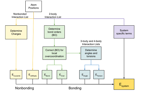
If you need to obtain the trajectory of all particles, according to Newton's motion equation, you need to know the initial position and speed of the particles, quality, and stress. The force of the particles is the negative gradient of the potential energy function, so in the molecular dynamics simulation, the potential energy function between all atoms must be determined, that is, the function of the momentum between the two atoms. Power field.

In molecular dynamics, the optimization of complex force field is an important issue. Reaxff is the representative. Compared with the traditional force field based on static chemical bonds and static charge assumptions that do not change with the chemical environment, Reaxff introduces the concept of key -level potential, which allows the keys to form and disconnect throughout the simulation process, and dynamically distribute charge for atoms. It is precisely because of the existence of these characteristics that the form of the reaction field is obviously more complicated than the classic force field. This makes it more difficult for us to perform the loss function obtained by the energy equivalent and density or density or experimental value comparison, as shown in Figure 2.

Figure 2 Parameter composition of the reaction force field

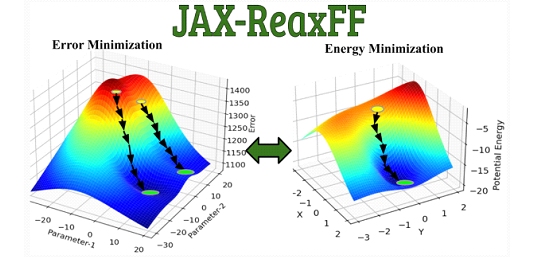
Various global optimization methods, such as genetic algorithms, simulation annealing algorithms, evolution algorithms, and particle group optimization algorithms, etc., often do not use any gradient information, which may make these search costs very expensive. The emergence of JAX brings possibilities for the solution of this problem.

Jax-reaxff:

1) Process

Figure 3 JAX-Reaxff process

Figure 3 is an overview of the task stream of JAX-Reaxff, which can be roughly divided into two stages: clustering and main optimization cycle. The main optimization cycle includes the energy minimization of the gradient information and the optimization of force field parameters.

As long as the cluster is performed according to the interactive list, the cluster is properly aligned in memory to ensure effective single instruction multi -data (SIMD) parallelization to improve efficiency.

The process of minimizing energy in the main optimization cycle is to find the process of the minimum energy and stable geometric configuration.Its specific approach is to optimize the gradient of atomic coordinates using JAX to find the system potential.The optimization of the force field parameters uses two ways to optimize the optimization of Newton in the original text-L-BFGS and SLSQP.This scipy.optimize.minimize function is implemented, where the function is directly introduced into the JAX solution gradient to improve efficiency.Energy minimization and force field parameter optimization iteration cycle.Figure 4 JAX-Reaxff main cycle optimization

Github address:

https://github.com/cagrikymk/jax- reaxff

2) Effect

The author has achieved parameter optimization on multiple data sets. It can be seen that compared to other algorithms, the optimization of JAX gradient information has a significant speed advantage.

Figure 5 Metal cobalt dataset results

references:

https://pubs.acs.org/doi/pdf/10.1021/acs.jctc.2c00363