The magnetism of matter is a simple but very subtle problem.Historically, magneticity was discovered very early.But strangely, the seemingly so powerful classic physics cannot describe such "simple" magnetism!Specifically, the conclusion of the application of classic electric power under the framework of statistical mechanics cannot give any magnetism!This difficulty was not resolved until the appearance and development of quantum mechanics in the 20th century.Only under the description of quantum mechanics can be given magnetic framework!This article attempts to explain why classic electric power cannot give magneticity through strict arguments.Then why can the quantum model be introduced by the quantum model to give magnetic and correct macro magnetic laws.Finally, explore a very strange nature of (quantum) limited energy -level magnetic system -negative temperature!
1 The statistical mechanics procedures cannot give material magnetism with statistical mechanics procedures
Consider a non -interaction N -granular system in the field.When there is only a magnetic field in the field, there is no electric field, the system given by the classic electric power Hamiton is:
< /g> < /g> < /g> g data-mml-node = "texatom" transform = "translate (503, -150) Scale (0.707) "data-mjx-texclass =" order "> < /g> < /g> Among them "stroke-width =" 0 "transform =" matrix (1 0 0-1 0) "> from the magnetic challenge Rotate gives:
< /g>
So the regular score function of the system is:
< /g> < /g> < /g> < /g> < /g> < /g> < /g> < /g> < /g> < /g> < / g> /> < /> < /> g> < /g> < /g> < /g> < /g> < /g> < /g> < /g> < /g> < /g> < /g> < /g> < /g> /g> > < /g> < /g> < /g> < / data-mml-node = "texatom" data-mjx-texclass = "order" transform = "translate (5548, 763.5)"> < /g> g data-mml-node = "texatom" transform = "translate (13376.2, 1476.6) scale (0.707)" data-mjx-texclass = "order"> < g data-mml-node = "mi" /> < /g> < /g> > < /g> g data-mml-node = "msup" transform = "translate (566, 0)"> < /g> < /g>
Note that the < /g> and < /g> Principles (uninterrupted in the same particle) and the principle of quantum uncertainty in the classic distribution function (equivalent to these two retained factors). However, because these two factors do not contain magnetic field , so in the calculation below, it is only an unimportant constant. Therefore
< /g> < /g> < /g> < /g> < /g> /g> Because Helmholtz is free and magnetic field It has nothing to do with it, so the system at any temperature The average magnetic torque is:
< /g> < /g> < /g> < /g> < /g> < /g> < /g> < /g> < /g> < /g> < /g> < /g> So classic electric power can not be magnetic in the framework of statistical mechanics!That is to say, there is no magnetic status in classic physics!
2 Under the description of quantum mechanics, the statistical mechanics procedure gives material magnetic 2.1 semi -classic model -the classic description of the spinning magnetic moment
Consider a N -granulated system.Each particle is at a grid point.Under the framework of quantum mechanics, if the interaction between coupling between magnetic torque and magnetic torque is not considered for the time being, the Hamilton volume of the magnetic system can be written:
< /g> < /g> < /g>
To simplify the reasons, first assume that a classic spin on each grid (that is, first assume that the magnetic torque You can in .data-mml-node = "math"> The regular distribution function of the system is:
< /g> < /g> < /g> < /g> < /g> < g data-mml-node = "mi"/> < /g> < /g> < /g> < /g> < /> < g data-mml-node = "texatom" transform = "translate (469, -150) scale (0.707)" data-mjx-texclass = "order"> < /> g> < /g> < /g> < /g> < /g> < /g> < /g> < /g> So the HELMHOLTZ free energy of the system Yes:
< /g> < /g> < /g> < /g> So the average magnetic moment of the system is:
< /g> < /g> < /g> < /g> < /g> < /g> < /g> < /g> < /g> < /g> < /g> < /g> < /g> < /g> < /g> Rect width = "1525" height = "60" x = "120" y = "220" /> < /g> < /g> < /g> "> < /g> < /g> When < /g> < /g> or < /g> (that is, at high temperature and low field), the average magnetic torque can be further simplified into:
< /g> < /g> < /g> < /g> < /g> < /g> < /g> < /g> < /g> < /g>/g> So the magnetization rate is:
< /> g data-mml-node = "mn" transform = "translate (1759, 0)"/> < g data-mml-node = "mrow" transform = "translate (220, 710)"> < /g> < /g> < /g> < /g> < /g> < /g> < /g> g data-mml-node = "mo" transform = "translate (14392.7, 0)" /> So this model gives magneticity and gives a magnetic (magnetic) property equation. The form of the material equation is exactly the same as the law of the law that met the magneticity of the magneticity measured by the macro experiment, that is, the inverse relationship between the magnetization rate and the temperature! So we have successfully derived the macro magnetic nature from this micro -model!
2.2 Puzzle Model -Quantum Description of Self -Spin Magnetic Magic
Although the (2.1) model gives the correct form of magnetic material equation, we noticed that the spin in this model is still classics )! So in order to get more accurate conclusions, we must replace it with a real quantum spin!
< /g> < /g> < /g>
< /g> < /g> < /g> < /g> < /g> < /g> < /g> < /g> < /> g> "Currentcolor" file = "Currentcolor" stroke-width = "0" transform = "matrix (1 0 0-1 0)"> < /g> < g data-mml-node = "mo" transform = "translate (1467.5, 0)" /> < /g> It is Bohl Magnetic. So the system of the system of the system is:
< /g> < /g> < /g> < /g> < /g> < /g> < /g> < /g> < /g> < /g> < /g> < /g> < /g> < /g> < /> < /> g> < /g> < /g> < /g> g data-mml-node = "mo" transform = "translate (6379.7, 0)" /> < /g> g data-mml-node = "mo" transform = "translate (1180.2, 0)" /> < /g> < /g> < /g> < /g> < /g> < /g> < /g> < /g> < /g> < /g> < /g> < /g> < /g> < /g> Rect width = "1001.2" height = "60" x = "120" y = "220" /> < /g> "> < /g> < /g> < /g> /g> Among them, the parameters is the magnetic field function:
So the helmholtz freedom of the system is:
< /g> < /g> < /g> < /g> < /g> < /g> < /g> < /g> < /g> < /g> < /g> < /g> < /g> < /g>Rect width = "1001.2" height = "60" x = "120" y = "220" /> < /g> "> < /g> < /g> < /g> So the average magnetic moment of the system is:
< /g> < /g> < /g> < /g> < /g> < /g. > < /g> g> data-mml-node = "mi" transform = "translate (736, 0)" /> < /g> < /g> < /g> < /g> < /g> < /g> < /g> < /g> < /g> < /g> /g> Note in the limit situation < G Stroke = "CurrenTColor" Fill = "Currencolor" Stroke-Width = "0" Transform = "MATRIX (1 0 0-1 0)"> (At this time, the quantum effect of spinning spatial spatial orientation disappears), the formula of the above average magnetic torque degrades into each composition is the classic spin:
< /g> < /g> < /g> < /g> < /g> < /g> < /g> < /g> < /g> < /g> /g> < /> g data-mml-node = "mi" transform = "translate (3380.7, 0)" /> < /g> < /g> g data-mml-node = "mo" transform = "translate (7041.9,
0) " < /g> < /g> < /g> When < g data-mml-node = "math"> or "> (that is, at high temperature and low field), . Therefore, the average magnetic torque can be further simplified into:
"> < /g>
For electrons without self-spin-orbit (L) coupling, , < /g> . Obtained in the upper formula: < /G> < /g> < /g>
Then get magnetization rate:
< /> g data-mml-node = "mn" transform = "translate (1759, 0)"/> < g data-mml-node = "mrow" transform = "translate (220, 710)"> < /g> < /g> < /g> < /g> < /g> < /g> /g> So after our model completely considers the quantization value of spining in the inner space, we still get the magnetic equation of the magnetic (smooth magnetic) of the previous form to meet the macro magnetic nature The law of Juli! But it is worth noting that because we consider the amount of spin on each grid point Sub -effect, so at this time, the Juli coefficient is three times the original! That is, after considering the quantum effect of the spin itself, the magneticity becomes larger!
3 (quantum) negative temperature characteristics in the limited energy -level magnetic system
Finally, let's discuss the strange characteristics of the negative temperature unique to the (2.2) (quantum) limited energy -level magnetic system! For the sake of simplification, we only take the two-capacity system without spin (s)-orbital (L) coupling as an example. At this time, < /g> < /g> < /g> < /g> CurrenTColor "Fill =" Currentcolor "Stroke-Width =" 0 "Transform =" Matrix (1 0 0-1 0) "> "> < /g> . Instead of in (2.2), the quantum regular score function and helmholtz free can expression Get the formula:
< /g> < /g> < /g> < /g> < /g> < /g>
< /g> and entropy = "Currentcolor" Fill = "Currentcolor" Stroke-Width = "0" Transform = "Matrix (1 0 0-1 0)"> dependence:
< g data-mml-node = "mi" /> < /g> < /g> < /g> < /> g data-mml-node = "mo" transform = "translate (7108.4, 0)" /> < /g> < /g> < /g> < /g> < /g>
< /g> < /g> < /g> < /g> < /g> < /g> < /> g> < /g> < /g> < /g> < g data-mml-node = "mi" /> < /g> g data-mml-node = "mi" transform = "translate (521, 0)" /> < /g> Temperature In turn, it is expressed as a function:
< /> g> < /g> < /g> < /g> g data-mml-node = "mo" transform = "translate (4012.7, 0)"/>
So can be expressed as function:
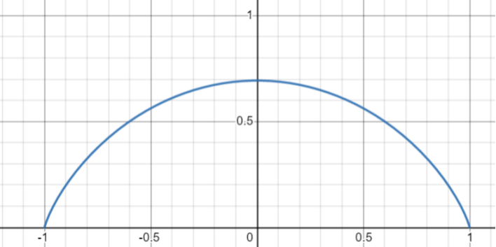
< /g> < /g> < /g> < /g> < /g> < /g> < /g> < /g> < /g> < /g> < /g> < /g> < /g> It is easy to find is Puppet function. In order to intuitively see and , Figure 1 made - Function Sketic Sketch:
Figure 1 -Entropy (S) -The functional relationship sketch of the functional relationship. The vertical coordinates are entropy, and the horizontal coordinates are internal energy
It can be seen that when you can When - The slope of the function is positive; when the inner can When it is greater than 0, - The slope of the function is negative. And - The slope of the function is exactly proportional to the inverse temperature, that is::
< /g> < /g> < /g>
The upper formula can be regarded as the temperature . It is easy to see < g data-mml-node="mi" />- Function slope positive and negative directly determines the positive temperature T positive burden! Therefore, U is less than 0 (that is, the left half of Figure 1) corresponding to the normal positive temperature (normal balanced state thermodynamic temperature). But U greater than 0 (that is, Figure 1 to the right) corresponds to negative temperature! Intersection At the negative temperature, because the internal energy is greater than 0, the high -energy level of the two -energy electronics system is more than the low -energy level, which means that the so -called "particle number reversal" is achieved! According to the Bolitzman distribution, the number of low -energy particles occupied by the system reaches to thermal balance must always be greater than the high -energy level (the number of particles of high and low energy at high and low energy at a high and infinite temperature is just equal). Therefore, in order to go to the high -energy level that exceeded half of the particle PUMP, the negative temperature is actually a temperature that is higher than the temperature that is infinite! Because the number of particles in negative temperature is in a reversal distribution, the negative temperature system is not a stable and balanced system. Most of the particles occupied by high energy levels will quickly jump down to low energy levels. This negative temperature system rarely appears in nature, but it can produce a lot of useful negative temperature systems through artificial manufacturing, such as laser. Edit: Shepherd
- END -