Basic relationship between quantum mechanics

The basic relationship between quantum mechanics is the right relationship between positions and its common momentum

This pairing relationship contains the core law of quantum mechanics, and is the most fundamental difference between quantum mechanics and classic mechanics. Similar to other physical theories, there is basically a development process for easy relationships. This development process is also the development process of matrix mechanics. This development process is very fast. Since the theory of Klames San was proposed in 1924, the three forms of the relationship between easy relationships, the germination form of Kun Thomas and the rules, and the transition form of the quantitative conditions of Heisenburg quantity conditions The modern forms of Bohn Johndong and Dirac both occurred in 1925. This article briefly introduces the theory of Krammers's San, and then introduces Kun Thomas Qiu and Rules, Haisenburg quantitative conditions and Bohn's contribution, and Dirac quantum Bousong brackets. At the end of this article, the process of matrix mechanics seeking hydrogenation atoms is briefly described, and the equivalent of volatility and matrix mechanics is more detailed.

1 Krammer San theory

The experiments of the Conopon effect have made people admit that the correctness of the Ainstein optical quantum theory, but this is bound to overthrow the existing electromagnetic theoretical system, and Maxwell's electromagnetic theory looks so unbreakable and cannot shake. In 1924, Bohr, Krammer, and Slyt published the theory of Boh Krammers Slyt (BKS) attempting to solve the dilemma of the continuity of the light waves and the discontinuity of the atomic transition [1]. From the perspective of BKS theory, when a atom is in a state, it will connect with other atoms through the radiation field. This virtual radiation field comes from the virtual vibrator with possible atomic transition frequency, which has the function of inducing atomic transition. Due to Bohr's negative attitude towards optical quantum, the BKS theory is not the contradiction between the volatility of the light and the particles, but to connect the continuous electromagnetic field and the discontinuous atom transition. The role of the virtual radiation field is to obtain the statistical energy and momentum conservation by determining the chance of transition of atoms, which means that the cause and effect description of the atom's radiation launch and absorption should be abandoned. As a result, BKS was concluded: Energy and momentum conservation was only established in a statistically sense, and the process of the GM is not strictly established. The cost of energy and momentum is too much, and it has been strongly opposed by Einstein, Paoli and others. In 1925, Bott, Conopaton and others independently denied the BKS theory from experiments, confirming that the element process energy and momentum conservation of photons and electron interactions were also accurately established [2,3]. They conducted a detailed study of the Convedon effect experiments. The experimental results showed that there were obvious similarities and perspectives in the existence of backbuilding electrons and scattered photons in Connpton scattering. Time and direction are random, and there is no significant similarities and angle correlation between the backbuilding electrons.

Although the BKS theory is denied, some of its thoughts are not meaningless. Krammes studied the phenomenon of scattered phenomenon with virtual Zhenzi's thoughts and achieved positive results. To this end, let's introduce the classic color scattered theory. A atom and a price electron are regarded as an electric puppet vibrator. When a bunch of polarized monochrome E = E0COS (2πνt) is illuminated by the atom, it will produce the same direction as the vaporization direction. Electricity moment

The equation that can be satisfied by Newton's second law

(1)

Mate M is electronic quality,

The frequency of Zhenzi's original signs. Formula (1) steady -state interpretation

(2)

If the atom has K species polarization and each polarization has FK electron, the polarization strength of the atom is

(3)

Therefore

(4)

The dielectric constant (4) dielectric constant α is linked to the refractive index of the atom to the light, so it is called the theory of the atomic response to light.

The above is the classic result of the atoms of light -colored scattered. In 1921, Laddenburg associated the intensity factor F of the classic scatter theory F and Einstein spontaneous radiation coefficient A to get

,in

H is Planck constant. Repair the classic forms (3) into quantum forms [4]

(5)

I in the formula (5) represents the atomic state, K represents the stimulus. This form of color scattered reflects the absorption of the atom's light, the atom absorbs light, and the atomic level is transformed from the base state I to the high energy level K. In 1924, Krammer promoted i as an exciting state, and rewritten the formula of the Ladenburg color scattered formula (5) to

(6)

in

[5]. The first connotation of the formula (6) is the same as that of the same formula (5). The second item represents the atom absorption of light, and the energy level of the atom is transitioned from high energy level to low -energy K ′. This negative absorption corresponds to Einstein's excitement. The second item of abnormal colors was later confirmed by a series of experiments by Ladenburg and others. In 1924, Klames, Bohn and Vanflek independently launched Krammer's scattered formula with the help of Bohr's corresponding principles (6) [6,7,8].

2 Basically sprouts for easy relationships: Kun Tomas seeks and rules

Affiliate

A (6)

(7)

Consider the limit situation

Formula (7) transition to the classic atomic jj Thomson =

So

(8)

This form is Ken Tomaas Qiu and Rules [9,10]. Kun and Thomas did not give further research results. They only needed a little forward to get a transition form that was basically easy to act: Haisenburg quantitative conditions, so Kun Tomas and rules can only be regarded as basically easy to Easy Easy Easy Easy Easy The form of bud in relationships. In fact, the principle of Bohr's corresponding principle, but the relationship between Einstein's spontaneous radiation coefficient and XKI [11]

(9)

The XKI in the formula is the position coordinate

The quantum physical quantity corresponding to the Fourier component X 的 is only related to two fixed state transitions.

For the physical quantity XKI's modulus, due to physical quantity | XKI | 2 and Einstein spontaneous radiation coefficient

In connection, it determines the intensity of the spectrum. The relationship between the formula (9) and the relationship between the bathbao is substituted to Kuntomas for the same (8)

The upper form is the condition of Haisenburg quantification.

The corresponding principles of Bohr will appear later. Here we will make more detailed explanations of the corresponding principles. The corresponding principle is an important contribution of Bohr during the old quantum theory. After the emergence of matrix mechanics, Bohr once said that the entire tool of quantum mechanics can be regarded as a precise expression of the tendency containing the corresponding principles. Boan also believes that the corresponding principle is a bridge from classic mechanics to vertical mechanics. What is the corresponding principle? In 1918, Bohr expressed this: there is no detailed theory about the transition mechanism between the state, of course, we cannot generally obtain the strict determination of the spontaneous transition rate between the two such fixed state, unless each of each n is some large numbers ... For those N values ​​that are not very large, there must be a close connection between the probability of a given transition and the Fourier factor in the two fixed state of particle displacement. [ 12].

From the perspective of Bohr's discussion, the main purpose is to try to find the relevant factors that affect the probability of transition, and there is a close connection between the probability of transition and grain (electrical) subtraction representation of Bohr's expression. It showed Boh's strong physical intuition, and later the quantum mechanics confirmed that the probability of transition was related to the transition amplitude corresponding to the classic Fourier coefficient. The close connection between the jumping probability between Bohr and the classic amplitude contains some important qualitative correspondence. For example, it can determine the situation of quantum transition to zero by analyzing the analysis of classic amplitude. In this way, he can export the choice of quantum transition, and the polarizing nature of transition radiation, which has great importance in the old quantum theory period. In the statement of Bohr's corresponding principle, "Unless N is a large number" provides people with a specific method of using the corresponding principles. The actual situation is usually used. The

a. When n ′ and n are large numbers, and they are much larger than N′-N, the frequency of transition radiation is basically (or a classic pan-frequency) of the classic winding frequency of the corresponding orbit. coincide. In particular, when N ′ and N are adjacent to the state, the frequency of transition radiation is basically equal to the classic winding frequency of the corresponding track.

b. Under the limit of the above -mentioned large number of sub -numbers, the chance of transition is proportional to the classic amplitude of the corresponding pan -frequency.

c. The above laws are not only established under the limit of a large number of sub -number, but also may be established under any quantum number. This situation is greatly guessing.

3 Basically transitional form of Easy Relation

In 1925, Krammes and Heisenburg adopted Bohn's approach, that is, after rewriting the micro -quotient of the actual amount J was rewritten into differentials, the completely quantum Kramurissenburg San formula was exported [13]

(10)

The physical significance of the quantum physical quantity XKI and its mold square | XKI | 2 is as mentioned earlier. In order to calculate the color scattered formula (10) | XKI | 2, you must figure out what is the physical essence of the quantum physical quantity Xτ corresponding to the position of the position coordinate x τ τ. The computing rules between XKI, especially the rules of the multiplication. Boline, Haisenburg, about the discussion after discussion that the multiplication of the physical quantity XKI is different from the multiplication of general physical quantities, but should abide by the rules of the unknown symbol multiplication rules. What is the mysterious symbolic multiplication rules? These problems were urgently needed to be resolved at the time, which was greatly important for the development of quantum theory at that time. In 1925 Heisenburg gigenically put the position coordinates

Return into a matrix, the matrix element is

In this way, the physical essence of the physical quantity XKI is the matrix element of the position coordinate (except for the phase factors related to time

), The symbol multiplication of the two physical quantities XKI is a simple matrix multiplication. Heisenburg solved the above problems and quickly created matrix mechanics [14,15].

A series of fixed state in Bohr's hydrogen atomic theory corresponds to one energy E (n), E (L), etc. The direct transition atom of the two energy levels will release a photon.

(11)

Formula

For the constant of the Planck. Obviously, the frequency of the Ritz is determined, that is,

(12)

The classic method is described by the amplitude and frequency to describe the movement, and the positioning of the position must be marked as the Fourier level

(13)

In the infinite range of 无 无, ω (n) is the base frequency, and τ ω (n) is a harmonious frequency. X (t) is the real number, so that the relationship X -τ = xτ*is established. Quantum theory of Zhonghaisenburg replace the position (13) to express the information of the atomic, the position coordinate matrix element is (14)

式（14）中l=n－τ为式（13）中的各项对应，并且假定x(l,n)=x(n,l)*和ω(l,n)=－ω(n, l) Establishment. Such a replacement is a leap of thinking. It introduces the matrix into quantum mechanics. The following analysis will see X (n, L) is an infinite dimension matrix.

How to multiply the two matrix x (n, l)? This requires the transition of the classic expression of X (T) 2 to the quantum expression. With the help of the Fourier transformation, the convolution is easy to get

in

(15)

From formula (14), formula (15) reasonably translated to the form of quantum theory

(16)

The form of Haysenburg (15) to the formula (16) is not unreasonable. The main reason is to meet the theoretical requirements of the Ritz combination (12) requirements. In fact, the light in the quantum theory is the result of the electrons in the atomic transition in the beginning and end. In the classic situation, the frequency relationship is τω (n)+(β -τ) ω (n) = βΩ (n). Regulations require that the quantum theory of quantum theory corresponding to the classic frequency relationship is ω (n, n -τ)+ω (n -τ, n -β) = ω (n, n, n -β), and press the corresponding correspondence of this foot label Relations, formula (15) must be transcribed into formula (16). It is known from the formula (16), and the square X (T) 2 of the position coordinates is also a matrix, and its matrix element is B (n, n, n -β) eiΩ (n, n -β) T. If it is two different physical quantities

y (t) =

By product, the classic form is

Formula

(17)

Formula (17) to translate to quantum theory as

(18)

The expression of the two physical quantity multiplication in quantum theory (18) is essentially the product of the two matrices in mathematics.

With the physical quantity in quantum theory is a brand new idea of ​​matrix, now examine the condition of Bohr Suofei quantification

(19)

There are new forms. To this end, we still start from the classic expression (13), and use the principles of Bohr to translate quantum conditions to quantum theory. From the formula (13)

Quantum theory conditions are expressed as

(20)

Use when you get the upper style

The requirements of Bohr corresponding to the principle, quantization conditions (19) cannot be consistent with quantum dynamics, and more naturally use the expression of quantum numbers to be slightly different.

Considering the formula (20), the formula is

(twenty one)

Now it is necessary to translate the formula (21) through the principle of Bohr to the quantum theory. Requirements corresponding to the principle of Bohr: When the number of main quantum N is large, the frequency of quantum frequency transitions to the classic frequency, that is,

Refer to Boh's frequency conditional formula (11)

F (n) in the upper formula is any function, that is, Bohr's corresponding principle requires that the classic situation Function F replaces the quantum number N micro -quantum into the form of differences in quantum theory. Haysonburg learned from Bohn to translate the formula (21) to a different form of color dispersion formula for Krammers or the discrimination form of Kun Tomas

(twenty two)

Formula (22) is the quantization condition of Heisenburg.

4 Basically to modern forms of relationships: the contribution of Boan and Jonodang

After Haysonburg published his new mechanics, Boan and Jonodang further developed the idea of ​​Haisenburg. The most important task they did was to rewrite the conditional condition of Haisenburg (22) to a more concise Form [16]. Bolosso Mo Fei quantitative conditional condition (19) can be written as

(twenty three)

The amount of role in the formula j = nh. Classic momentum, position expression is p =

Obviously

The formula (23) of these expressions is substituted into the quantitative condition (23) and the two sides of the equation are divided into J

(twenty four)

I used the relationship when I got the upper formula

Note that J = NH is known from the corresponding principle that the translation of the formula (24) to the quantum theory has the following form.

(25)

Physical quantity P, Q are matrix in quantum theory, formula (25) indicates that the PQ -QP matrix is ​​diagonal matrix, and its diagonal (PQ -QP) nn is

Formula (25) can be written as a concise form as follows

(26)

Formula

It is the constant of the Planck, i is an infinite -dimensional unit matrix. Since the location and momentum are matrix, and

The matrix where the location and momentum change over time are q (t) =

The matrix element of Q (T), P (T) is substituted (25)

This result is the conditional condition of Haisenburg quantification (22). Bohn and Jonang use Q to indicate the position coordinates. The ease relationship between the position coordinates and its co -consuming momentum (26) is the basic relationship between quantum mechanics. Boan believes that the export of this relationship is the most important discovery of his life. Dirac also got the style (26) from the quantum pine brackets, but it was a little later than Bohn.

5 Basically, modern forms of relationships: Dirak quantum Poor brackets

In September 1925, Dirac's mentor R. No Le received the articles (one person article) that can be used to establish matrix mechanics based on the corresponding principles of Heisenburg based on the corresponding principle. Dirac's attention was attracted by the mysterious mathematical relationship in the Haysenberg's article. A few weeks later, Dirac returned to Cambridge University and suddenly realized that the mathematical form and classic mechanics in the Hemansberg article Poison brackets have the same structure. Starting from this idea, Dirac quickly developed the quantum theoretical quantum pine brackets based on non -transmitting dynamic variables. How can two quantum physical volume transition to their classic pine brackets? According to Heisenburg's point of view, the volume X and Y in quantum mechanics should have matrix forms. The volume of two mechanics volume does not meet the exchange law, that is, XY ≠ YX. In order to facilitate the use of the corresponding principle, assuming the number of quantum N (n, n -α) of the X matrix N is large, and α is much smaller than N. In this way, the matrix element of x can be briefed as x (n, n -α) = xαk, jr = nrh, H is the Planck constant, the angle bid R represents a pair of co -variables: the actual volume variable J and angle variables W = ωt/2π degree of freedom. The classic corresponding to M = N -α -β, the classic of the matrix element (xy -yx) nm of XY -YX is

(27)

n is a large number of sub -numbers, α, β is a small quantum number that jumps between the initial and last state. -X (n -β, n -β -α) =

Similarly, the second item of the formula (27). Notice

Available

Therefore, the classic correspondence of XY -YX's matrix element (xy -yx) NM can be transformed into

(28)

In the formula (28), alpha, β are small quantum numbers, n, m is a large number of sub -numbers at the beginning and end, α+β = n -m is the constraint condition. Various possible transitions, the second sum of the sum of the sum of the sum of the freedom of JR and WR. XY -YX's overall matrix corresponds to -

Various possible transitions between the early and the end of the formula (28) have been included in the matrix multiplication. We get further

(29)

The PR and QR in the formula are any pair of covarrings of the system. As the classic Poor loader remains unchanged under the regular transformation, the formula (29) is established, that is, the XY -YX matrix in the quantum mechanics in a large number of subcurrents corresponds to

Take the classic Patson parentheses {x, y}, Dirac further assumes that the two are equal in any quantum number according to the principle of Bohr's corresponding principle.

(30)

From the classic Poor (QI, PJ} = ΔIJ of the classic Poor (Qi, PJ}, Dirac got the basic relationship between the quantum mechanics that Bohn and Yuedang had obtained

Haisenburg, Bohn, about the three people completed the complete expression of matrix mechanics [18], gave the arithmetic Hyenburg sports equation, thereby establishing a complete matrix mechanics. In fact, all the reasonable functions that set f as position Q and momentum p are obtained by basic relationships (26)

(31)

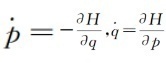
Make f equal to the system Hami volume H, Hamiton regular equation

The formula (31) becomes

(32)

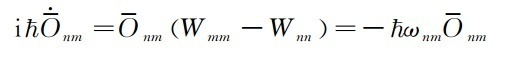
In this way, all are P, Q with rational functions o (p, q).

(33)

This form is the Hyenburg Movement equation of the arithmetic O.

6 Use matrix force to learn hydrogen dissolving atoms

In modern terms, matrix mechanics is the quantum mechanics of the energy appearance in the painting of Heisenburg. The Rune Haysenburg Movement equation is also a matrix equation. Matrix mechanics processing quantum mechanics problems, generally diagonally diagonally of the system's Hamiton, that is, W = SHS -1, S in the formula is the transformation matrix, W is the diagonal Hami meal, and the diagonal matrix matrix matrix. Yuan is the system's energy signs. An arbitrarily requires a corresponding regular transformation, that is,

After the transformation

(34)

Take the (NM) matrix element on both sides of the formula (34), and consider W as a diagonal matrix

have to

(35)

The solution of the formula (35) is

(36)

The relationship between the matrix of the arithmetic O is the change of time

(37)

It can be seen that the relationship between the maths in matrix mechanics is relatively simple. Specific physical problems are often proportional to the model of the motto element of the mechanical amount. For example, the strength of the spectrum is the same as the modgee of the atomic matrix element | RNM | 20 %. The main task of matrix mechanics is to obtain the system's energy signs to obtain the system's energy -based value through regular transformation. How to diagram the system of the system by transforming? Generally, first find the system that the system is paired with each other, and take these mechanics as a common appearance, then these mechanics has a certain value at the same time, and then according to the amount of the relationship between the ease and a certain amount of mechanics exported by the basic relationship, the amount of mechanics exported by the basis of the ease relationship and the certain amount of the amount of mechanics exported by the easy relationship and a certain amount of some of the amount of mechanical amount and a certain amount of some of the amount of mechanics exported by the easy relationship and a certain amount of some of the amount of mechanics and a certain amount of some of the amount of mechanics exported by Easy Relationships. The modulus of the mechanical quantity matrix element is more than equal to zero -obtaining the quantum quantization of these mechanics. Using matrix mechanics can obtain (J2, JZ) the lower angle of the appearance of the dynamic volume square J2 and the angle volume of the angle amount in the Z direction of JZ [19]

In the formula J =

In early 1926, Poly used the Donaldian-Lengdi vector to diagram the amount of hydrogen atomic Hanton, which obtained the Bohl formula of hydrogen atomic energy. Not only that, Paoli also easily solves the division of the hydrogen atomic spectrum under the action of the Stark effect and the cross -rail of Stark, and the problem of the hydrogen atomic spectrum. This problem has always been difficult to overcome the difficulty of the old quantum theory [20]. Our reference [21] summarizes the process of Pauli's hydrogenation atomic Boer Energy formula. The hydrogen atom in Hamilton is an electronic quality in the type, P is an electronic amount, and the coefficient A = E2/(4πε0). The total energy of the restrained hydrogen atom is less than zero. Jung Leng's secondary vector is K =

In the formula of the electrons, the orbital angle volume of the electrons, R is the position of the electron, the Jung asylum vector and the Hamilton quantity are ease [k, h] = 0 means that the vector is conservation. The Easy Relationship of the Rygeri Sub -vector is satisfied with

Define the new calculation vector

It can prove that j of satisfaction is the same as the relationship between easy relationships and corner motion satisfaction, that is,

(38)

The relationship between Jung Leng's secondary vector and hydrogen atomic energy is

Based on the expression of the above A, J and K2, we get it

Then the amount of hydrogen atoms in Hamiton is

From the formula (38), we know

Among them, J is taken for integer or half, and (2J+1) must be natural numbers, so that (2J+1) ≡N. So the energy -level formula of the hydrogen atom is

That is the Booneng format for hydrogen atoms. Xue Dingzheng also derived the Bohneng -grade formula of the hydrogen atom from his volatility, but a few days later than Paoli. Dirac also studied hydrogen atoms and partially solved the energy -level problem of hydrogen atoms, and it was a little later than Paoli.

It should be explained that matrix mechanics requires a high skill to find and build a suitable physical quantity through regular transformation. It is very limited, such as one -vibration, corner movement, and hydrogen atoms are accurate solution systems. In fact, there are very few systems of volatility accurate solution. What is more important is to make a regular transformation of the system Hami Latin W = SHS -1. In addition to being able to directly obtain the energy signs of the eliminated system, it can also make a micro -disturbance calculation of the disturbing system, such as non -simplified micro -disturbances, micro -disturbances, and micro -disturbances, and miles. Simple disturbances and even timely disturbances, so that matrix mechanics can solve most of the problems of quantum mechanics. Due to the perspective of the amount of mechanics, matrix mechanics is difficult to solve the problem of time evolution, such as scattering. Volatility can easily deal with scattering problems. When dealing with specific problems, volatility is often much simpler than matrix force. This is also the main reason why volatility can surpass matrix mechanics and is more easily accepted by people.

7 The equivalent of volatility and matrix mechanics

In 1926, Xue Dingzheng, Paoli, and Ecart independently proved the equivalent of volatility and matrix mechanics. We used Xue Dingzheng's thinking to confirm the equivalent of the two mechanics from the following aspects [22].

Xue Dingzhang's equation is the motion equation that the wave function is satisfied in the painting scene of Xue Dingzhang. The motion equation of the Hassonburg is a motion equation that is satisfied with the calculation symbols in the painting scene. They are the basic equations of quantum mechanics. Because there is a transformation relationship between the two paintings, we can "derive" the Haysenburg sports equation from Xue Dingzhang's equation. In the painting scene of Xue Dingzhang's painting, the amount of force does not show time OS,

The wave function changes over time

The wave function follows Xue Dingzhang equation

The wave function at any moment

In the painting scene of Heisenburg's painting, the relationship between the amount of mechanical quantities changes with time.

The wave function of Haisenbao's painting scene does not change with time

As a result

The equation that the wave function meets

Any two mechanics in matrix mechanics multiplied to meet the matrix multiplication

Volatility can prove it. In fact, take a set of orthogonal to one foundation U1 (Q), U2 (q), U3 (Q), ..., two mechanics matrix elements in the coordinate space

Obtain

The proposal was obtained. In the process of proved, we used the complete relationship between the Famian, the Emi nature of the F, and the base of the G arithmetic.

The matrix force has a basic relationship, and the volatility can also prove this relationship. The amount of motion in the coordinate space is as an arithmetic symbol, so the dynamic calculation arithmetic and coordinate Q computing symbol PQP =

Take a set of orthogonal to one foundation U1 (Q), U2 (Q), U3 (Q), ..., the coordinate matrix element is q (ln) =, so have to

The above formula is the basic relationship between matrix mechanics. In the process of proved, we used the position of the position of the position of the position, the momentum of the momentum, and the completeness of the foundation.

You can also use the volatility to prove the matrix of the Heisenburg Sports equation of the Matson Matrix

In the formula, the matrix of the amount of mechanics is under energy appearance, and W is the amount of diagonal Hami. To this end, the basements are taken in the coordinate space to complete the base of the base, U2 (q), u3 (q), ... as the function of energy, then there is

(39)

The basic assumptions of matrix mechanics

The frequency of moving in the formula meets the Bohr frequency condition

Therefore

(40)

From the formula (39) and the formula (40), we have obtained the Heisenburg Movement equation of the mechanical quantity matrix

Then, the Heisenburg Sports Equation, which gets the mechanical quantity matrix

From the above demonstrations, Xue Dingzheng's fluctuations and Haisenburg, Bohn, and Jonaldo are indeed equivalent.

8 conclusion

Compared with volatility, Edantttebroy Xue Dingzhang's clear and simple development line, the development of matrix mechanics is very complicated and twisted, and there are also genius inspiration and wisdom everywhere. The development process is very necessary, this is one of the main tasks of this article. This article introduces the background of matrix mechanics to the basis of matrix mechanics and the inspiration and work of the creation of quantum mechanics, and the three forms of basis of the development of relationships are explained in detail: library Endomas seeks the germination form of the rules, the transition form of the quantization conditions of Heisenburg, and the modern form of Bohnjon and Dirac. In order to deeply understand the quantum mechanics, including the method of matrix mechanics treatment, and the internal connection of the fluctuation and matrix mechanics, this article also briefly introduces the process of matrix mechanics to demolish the atom of hydrogenation, which expounds the volatility and matrix mechanics in detail. Equivalent. Boh hydrogen atomic theory failed to give information about the strength, line width, polarization and other information of the spectrum, and Boh asked his student Krames to study this problem. The intensity of calculating the spectrum should be used in Einstein's spontaneous radiation coefficient. The relationship between the scattered strength factor and Einstein spontaneous radiation coefficient when the color dispersion phenomenon is found in bondenburg. The phenomenon of color dispersion is linked with the energy level transition of quantum. Krammers promoted the scattered results of the Ladenburg and successfully established the Clames Sanda theory. Kun and Thomas transitioned the Krameris Sanda formula to the classic JJ Thomson Sanda formula from the corresponding principles, and got Kane Tomas seeking and rules. As described in the article, this harmonious rule is a bud that basically the relationship between easy relationships. Hesonburg and Krammes collaborated to get a completely quantum Kramurissenburg San formula. In this formula, the quantum physical quantum XKI corresponds to the position coordinate Fourier component Xτ. The physical essence of the physical quantity XKI is the matrix element of the position coordinates. As a result, the transitional form of the basic relationship is established: Hyenburg quantification conditions. Although the conditions of Haisenburg quantification are not a modern form of easy -to -ease relationships, it is the beginning of matrix mechanics and a breakthrough in the concept of quantum mechanics, because Haisenburg clearly introduces matrix into quantum mechanics. We also see that the research of atoms on the theory of light color scattered directly leads to the birth of matrix mechanics. Boan and Jonodang fully followed the road of Heisenburg, and obtained a modern form of quantum mechanics basically easy -to -relationship. Dirac was inspired by the Haysenburg matrix mechanics articles. The incompetence of the matrix multiplication was easy to think of the classic Patson parentheses. Essence With a basically easy relationship, establishing the entire matrix mechanical system is logical.

references

[1] Bohr n, Kramers H, Slater J. The Quantum theory of Radiation [J]. Philosophical Magazine, 1924, 47: 785-802.

[2] BOTHE W, Geiger H.über Das WESEN des ComptoneFFEKTS; Ein Experimenteller Beitrag Zur theorie Der Strahlung [J]. Zeitschrift für physik, 1925, 32: 639-663.

[3] Compton a, Simon A. Direct Quanta of Scattered X-Ray [J]. Physical Review, 1925, 26: 289-299.

[4] Ladenburg R. Die Quantentheoretischedeutung Der Zahl Dispersionselektronen [J]. Zeitschrift Für Physik, 1921, 4 (4): 451-468.

[5] Kramers H. The Law of Dispersion and Bohrs Theory of Spectra [J]. Nature, 1924, 113: 673-674.

[6] Kramers H. The Quantum theory of dispctions [j]. Nature, 1924, 114: 310-311.

[7] Born M.über Quantenmechanik [J]. Zeitschrift Für Physik, 1924, 26 (1): 379-395.

[8]VAN VLECK J. The absorption of radiation by multiply periodic orbits and its relation to the correspondence principle and the Rayleigh-Jeans law[J]. Physical Review, 1924, 24: 330-365.[9]KUHN W.Über DIE GESAMTSTSST gRKE DER VON Einem Zustande

AUSGEHENDEN ABSORPTIONINIEN [J]. Zeitschrift für physik, 1925, 33 (1): 408-412.

[10] Thomas W. über Die Zahl Dispersionselektronen, Die Einem Stationren Zustande Zugeordnet Sind (VORLUFIGE MITTEILUNG) [J]. Naturwissenschaften, 1925, 13: 627.

[11] Zeng Jinyan, Kazakhstan. The role of the corresponding principle in the development of quantum theory [J]. University Physics, 1985, 1 (9): 10-14.

Zeng J Y, Ka X L. The Role of the Principle of CorresPondnce in Quantum theory [J]. College Physics, 1985, 1 (9): 10-14. (In Chinese)

[12] Bohr n. On the quantum theory of line-specra [j]. D. kgl. Danske vidensk. SELSK. SKRIFTER, naturvidensk. OG Mathem. AFD.8. Række, 1918, IV.1: 1-3.

[13] Kramers H, Heisenberg W. über Die Streuung Von Strahlung Durch Atome [J]. Zeitschrift Für Physik, 1925, 31 (1): 681-708.

[14] Heisenberg W. über QuAntentheoretische UmDeutung KineMatischer Und Mechanischer Beziehungen [J]. Zeitschrift für physik, 1925, 33 (1): 879-893.

[15] Huang Yongyi. The development of the basic concept of quantum mechanics [M]. Hefei: Chinese University of Science and Technology Press, 2018: 42-46.

[16] Born M, Jordan P. Zur Quantenmechanik [J]. Zeitschrift Für Physik, 1925, 34: 858-888.

[17] Dirac P. The Fundamental Equations of Quantum Mechanics [J]. Proceedings of the Royal Society of London, Series A, 1925, 109: 642-653.

[18] Born M, Heisenberg W, Jordan P. Zur Quantenmechanik II [J]. Zeitschrift Für Physik, 1926, 35: 557-615.

[19] Zeng Jinyan. Quantum Lower Volume 1 [M]. 2 Edition. Beijing: Science Press, 1997: 401-406.

[20] Pauli W. über Das Wasserstoffspektrum Vom StandPunkt der Neuenteenmechanik [J]. Zeitschrift Für Physik, 1926, 36: 336-363.

[21] Qian Bochu, Zeng Jinyan. Selection and analysis of quantum learning questions (Book) [M]. Beijing: Science Press, 1999: 169-175.

[22] Schrgdinger E. über Das Verhältnis Der Heisenberg Born Jordanischen MEINEN [J]. Annalen der physik, 79: 734-756.; Xi'an Jiaotong University "famous teachers, famous courses, famous textbooks" construction project (school 2018); Xi'an Jiaotong University's second batch of "curriculum ideological politics" demonstration curriculum project (school 2019).

About the author: Huang Yongyi, male, associate professor of Xi'an Jiaotong University, mainly engaged in atomic physics teaching and research, [email protected].

Citation format: Huang Yongyi. The basic relationship between quantum mechanics [J]. Physics and engineering, 2021, 31 (1): 8-16.

- END -